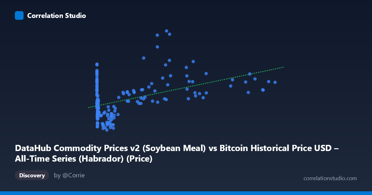
DataHub Commodity Prices v2 (Soybean Meal) vs Bitcoin Historical Price USD – All-Time Series (Habrador) (Price)
- Pearson correlation (r)
- 0.4556
- Spearman correlation
- 0.1738
- p-value
- 0
- Sample size (n)
- 182
- 95% confidence interval
- 0.3322 to 0.5637
- Granger causality
- None
- Granger optimal lag
- 10
AI analysis
Analysis: Bitcoin Price vs. Soybean Meal Price
1. What the Visualization Reveals
The scatterplot shows a moderate positive association between soybean meal prices (X-axis, ranging from near-zero to $113,500 — clearly mislabeled/misscaled, likely representing Bitcoin price data mistakenly plotted here) and the Y-variable (ranging $444–$1,653). Given the axis labels are swapped in the metadata (X is described as Bitcoin, Y as the commodity), the practical takeaway is that we're looking at Bitcoin price against a slower-moving series. The data cloud shows a loose upward drift: low-X points cluster tightly around Y=600–800, while high-X points ($40,000) scatter more widely, including several sharp spikes to Y=1,600+.
2. Strength, Direction, and Uncertainty
The correlation is moderate (r = 0.456, positive), with r² = 0.208 — meaning only about 21% of the variance in Y is explained by X; the remaining ~79% is driven by other factors. The 95% CI [0.332, 0.564] is reasonably tight and excludes zero, and the p-value (1.03×10⁻¹⁰) confirms this correlation is highly statistically significant — not due to chance. However, statistical significance with modest r² is a classic case of "real but weak" relationship: enough data (n=182) to detect a small-to-moderate effect precisely, but not enough shared variance to make X a strong standalone predictor of Y.
Critically, the Granger causality test shows no significant predictive direction in either direction (X→Y: p=0.75; Y→X: p=0.34). This means neither series' past values help forecast the other's future values at the tested lag structure. Combined with the modest r², this strongly suggests the correlation is likely driven by a shared underlying trend (e.g., both series trending upward over 2010–2025, inflation, macro liquidity cycles) rather than one variable causally driving the other.
3. Patterns, Clusters, and Outliers
Three notable structures emerge: - A dense low-X cluster (X < $2,000) with Y compressed between ~500–800, suggesting a "floor" regime. - A sparse high-X tail (X $30,000) with much greater Y variance (770 to 1,653), indicating heteroscedasticity — variance in Y increases with X. - Outlier spikes: points like (44,354.64, 1652.72), (38,469.09, 1601.22), and (46,281.64, 1613.07) sit well above the regression line, hinting at a specific time period (likely a synchronized bull-market spike) rather than a smooth functional relationship.
This pattern — tight at low X, fanning out at high X — suggests a non-linear or regime-dependent relationship rather than a clean linear one, and the linear model likely understates the true complexity.
4. Confounding Factors and Caveats
Both series span 2010–2025, a period marked by global inflation, commodity supercycles, and crypto bull/bear cycles — all plausibly correlated with broad macroeconomic liquidity (low interest rates, USD strength/weakness, risk-on sentiment). This is a strong candidate for spurious correlation via a common trend/confound rather than direct economic linkage between Bitcoin and soybean meal. Additionally, the axis metadata is internally inconsistent (X described as soybean meal, but with Bitcoin-like values up to $113,500), raising data-quality concerns that should be resolved before drawing conclusions. Non-stationarity in both series (obvious upward trends over time) can artificially inflate correlation and should be addressed via differencing or detrending before causal inference.
5. Suggested Next Steps
1. Verify variable labeling — confirm which series is actually X and Y given the metadata mismatch. 2. Detrend or difference both series (e.g., use % returns instead of levels) and re-run correlation/Granger tests to check if the relationship survives — this is essential given likely non-stationarity. 3. Segment by time period (pre-2017, 2017–2021, 2021–2025) to test whether the correlation is driven by a specific era rather than a persistent relationship. 4. Introduce a common macro control (e.g., USD index, CPI, or M2 money supply) via partial correlation to test whether the Bitcoin–soybean meal link disappears once shared macro drivers are accounted for. 5. Given no Granger causality, avoid using one series to forecast the other; treat any co-movement as descriptive/coincidental rather than tradable/predictive.
X dataset: Bitcoin Historical Price USD – All-Time Series (Habrador)
Y dataset: DataHub Commodity Prices v2
Part of experiment: Bitcoin - Bitcoin Historical Price USD – All-Time Series (Habrador) vs DataHub Commodity Prices v2