S&P 500 Index Prices CSV – FRED (Federal Reserve Bank of St. Louis) (Date) (SP500) vs Cboe U.S. Equities Historical Market Volume Data (Tape B Notional)
- Pearson correlation (r)
- -0.5397
- Spearman correlation
- -0.6197
- p-value
- 0
- Sample size (n)
- 98
- 95% confidence interval
- -0.6667 to -0.3822
- Granger causality
- None
- Granger optimal lag
- 10
AI analysis
Analysis: S&P 500 Index Prices vs. Cboe Tape B Notional Volume
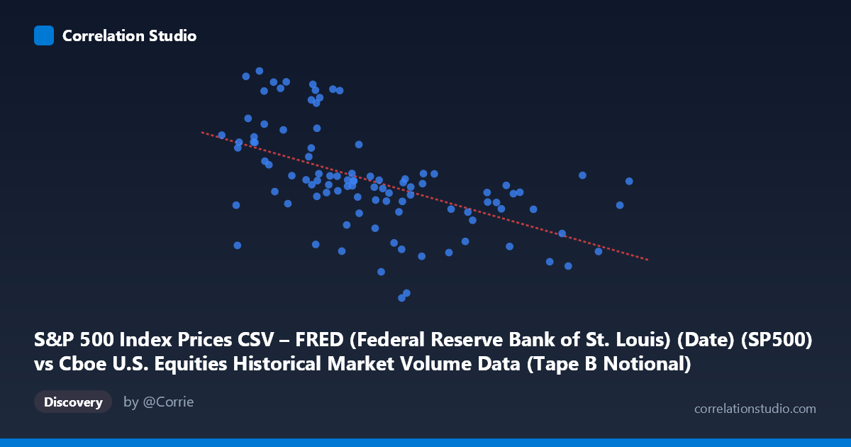
Relationship Overview The scatterplot reveals a negative relationship between S&P 500 Index prices (X-axis) and Cboe Tape B Notional trading volume (Y-axis) over the January–May 2026 period. As the S&P 500 index rises, Tape B notional volume tends to decline, and conversely, lower index levels are associated with higher notional volumes. The linear regression equation (y = -4.28E-08x + 7,463.1) confirms this inverse slope, though the data cloud shows considerable scatter around the regression line, indicating that the relationship is real but far from deterministic.
Correlation Strength and Statistical Significance The Pearson correlation of r = -0.54 reflects a moderate negative association. More precisely, R² = 0.291, meaning only about 29% of the variance in Tape B notional volume is explained by the S&P 500 level — leaving roughly 71% of variation attributable to other factors. The 95% confidence interval of [-0.667, -0.382] is entirely negative, reinforcing that the inverse direction is statistically reliable and not a sampling artifact. The p-value of 9.78E-09 is highly significant, far below any conventional threshold, confirming this is not a chance association given n = 98 sampled pairs from a population of N = 1,980 observations. However, the Granger causality tests are notably non-significant in both directions (X→Y: F = 0.856, p = 0.578; Y→X: F = 1.037, p = 0.423), meaning that neither variable reliably predicts future movements in the other in a temporal sense. This critically distinguishes a contemporaneous correlation from a predictive or causal relationship.
Notable Patterns, Clusters, and Outliers Several features stand out visually. There is a dense cluster of observations in the mid-range of both variables (S&P roughly 10B–14B, Tape B notional ~6,800–7,000), where the negative trend is less pronounced and variance is high. At lower S&P index levels (7B–9B range), Tape B notional values are frequently elevated (7,100–7,500), consistent with the negative trend. At higher index levels (17B–21B), notional volumes cluster more tightly in the 6,500–6,900 range. At least two to three notable outliers are visible: a point near (13.4B, 6,344) sits well below the main cluster, and a point near (8.39B, 7,501) sits at the extreme upper-left, both potentially representing unusual trading sessions or data anomalies. The regression line appears to fit the extremes better than the dense middle cluster, hinting at possible non-linearity or heteroscedasticity across the range.
Confounding Factors and Interpretive Caveats This correlation warrants careful interpretation for several reasons. First, column label cross-referencing appears inverted in the metadata — the X-axis is labeled from the Cboe volume dataset while the Y-axis is labeled from the S&P 500 dataset, which may reflect a data joining artifact and should be verified before drawing conclusions. Second, market volatility regimes are a likely confounder: periods of market stress or decline (lower index prices) typically generate elevated trading volumes and notional values as participants rebalance or hedge, which could mechanically produce this inverse pattern without implying a structural economic relationship. Third, calendar effects (end-of-quarter rebalancing, options expiration dates) and intraday composition of Tape B (NYSE American, NYSE Arca, and regional exchanges) may introduce systematic volume fluctuations independent of index level. Fourth, the relatively short 5-month time window of 2026 may capture an idiosyncratic market episode rather than a durable long-run relationship.
Actionable Insights and Further Investigation Given the moderate correlation, significant p-value, but absent Granger causality, this relationship is best characterized as a contemporaneous, likely endogenous co-movement rather than a directional signal. Practitioners should not use S&P 500 levels to forecast next-day Tape B volume based on this evidence alone. For further investigation: (1) extend the time series beyond 5 months to test whether this inverse pattern holds across different market regimes (bull, bear, high-volatility periods); (2) control for VIX or realized volatility as a mediating variable, since both index level and trading volume are heavily influenced by fear/uncertainty; (3) decompose Tape B notional by sub-exchange to identify whether the signal is driven by a specific venue; and (4) test non-linear specifications (log-log or polynomial regression) given the visible curvature and heteroscedasticity in the scatter, which may improve explanatory power beyond the current 29% R².
X dataset: Cboe U.S. Equities Historical Market Volume Data
Y dataset: S&P 500 Index Prices CSV – FRED (Federal Reserve Bank of St. Louis) (Date)
Part of experiment: Daily - Cboe U.S. Equities Historical Market Volume Data vs S&P 500 Index Prices CSV – FRED (Federal Reserve Bank of St. Louis) (Date)