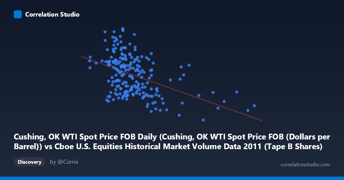
Cushing, OK WTI Spot Price FOB Daily (Cushing, OK WTI Spot Price FOB (Dollars per Barrel)) vs Cboe U.S. Equities Historical Market Volume Data 2011 (Tape B Shares)
- Pearson correlation (r)
- -0.4558
- Spearman correlation
- -0.437
- p-value
- 0
- Sample size (n)
- 212
- 95% confidence interval
- -0.5564 to -0.3421
- Granger causality
- None
- Granger optimal lag
- 1
- Time coverage
- 2011-01-03 to 2011-12-30
- Recomputed on refreshed data
- 2026-11-13 (r was -0.4558)
AI analysis
Analysis: WTI Crude Oil Price vs. Cboe Tape B Share Volume (2011)
Relationship Overview
The scatterplot reveals a moderate negative relationship between WTI crude oil spot prices (X-axis) and Cboe Tape B share volumes (Y-axis) across 252 trading days in 2011. As oil prices rise, Tape B equity trading volumes tend to decline, and vice versa. The linear regression equation (y = -1.14472E-07x + 106.116) confirms this inverse slope, suggesting that for every $10/barrel increase in WTI prices, Tape B volumes decrease by roughly 1.14 shares (in billions, given the scale). The relationship is visible in the point cloud's downward drift, though the scatter is substantial, indicating this is far from a deterministic relationship.
Correlation Strength and Statistical Significance
The correlation coefficient of r = -0.4664 indicates a moderate negative association. However, the coefficient of determination (r² = 0.2176) is the more practically meaningful figure — only ~21.8% of the variance in Tape B volumes is explained by WTI prices, leaving roughly 78% attributable to other factors. The 95% confidence interval of [-0.5579, -0.3638] is entirely negative and does not cross zero, confirming directional consistency. The p-value of 5.107E-15 is extraordinarily small (well below any conventional significance threshold), meaning this correlation is almost certainly not a chance artifact given the sample of 252 observations drawn from a population of 3,780. That said, statistical significance should not be conflated with practical significance — the relationship is real but modest. Critically, Granger causality tests show no significant predictive directionality in either direction: X→Y (F=0.0298, p=0.863) and Y→X (F=2.861, p=0.092) both fail to reach significance at the 5% level. This means that while prices and volumes are contemporaneously correlated, neither reliably predicts the other one period ahead.
Notable Patterns, Clusters, and Outliers
Several structural features stand out in the sample points. There is a loose clustering of observations in the 60–110 million barrel-price range with Tape B volumes between 85 and 105, forming the bulk of the point cloud. However, there are notable high-volume outliers at lower price levels — for example, (62,070,481, 111.68) and (101,941,452, 110.60) represent unusually high Tape B volumes relative to the general trend, pulling against the regression line. Conversely, several high-price observations (e.g., 169,125,865 at 93.96; 176,544,228 at 97.99; 189,743,290 at 85.48) cluster at lower-to-mid volumes, broadly consistent with the negative trend. There also appears to be non-trivial vertical dispersion at any given X value, suggesting the relationship is noisy and potentially non-linear in portions of the price range — a polynomial or piecewise model may fit better than a simple linear one.
Confounding Factors and Caveats
Several important caveats apply to this analysis. First, 2011 was a volatile year for both oil markets (Arab Spring, Libyan supply disruptions drove WTI toward $113/barrel) and equity markets (U.S. debt ceiling crisis, European sovereign debt fears), meaning both series were simultaneously influenced by major macroeconomic and geopolitical shocks — a classic common-cause confound. Second, Tape B specifically covers NYSE American (AMEX) and regional exchange-listed securities, which may be more sensitive to energy-sector equities, creating a compositional bias. Third, the absence of Granger causality warns against any causal narrative; the correlation likely reflects shared sensitivity to risk-off/risk-on macro regimes rather than a direct price-to-volume mechanism. Fourth, daily data introduces autocorrelation within each series, which can inflate effective sample sizes and make p-values appear more significant than they truly are on an independent-observation basis.
Actionable Insights and Further Investigation
Given these findings, several investigative paths are worth pursuing. Regime analysis — segmenting the year into identified macro stress periods (e.g., pre/post-August 2011 debt ceiling crisis) — could reveal whether the correlation strengthens during risk-off episodes and weakens during calmer periods. Analysts should also test alternative lag structures beyond lag-1 in the Granger framework, as oil price shocks may propagate to trading behavior over weekly rather than daily horizons. Including additional control variables (VIX, S&P 500 returns, USD index) in a multivariate regression would help isolate the oil-price effect from broader market sentiment. Finally, examining whether Tape A and Tape C volumes show similar or divergent patterns would clarify whether the relationship is broad-based or specific to Tape B's issuer composition, potentially informing sector-specific trading strategies around commodity price movements.
X dataset: Cboe U.S. Equities Historical Market Volume Data 2011
Y dataset: Cushing, OK WTI Spot Price FOB Daily
Part of experiment: Daily - Cboe U.S. Equities Historical Market Volume Data 2011 vs Cushing, OK WTI Spot Price FOB Daily