Nonfarm Payroll Employment (PAYEMS) (PAYEMS) vs Bitcoin Historical Price USD – All-Time Series (Habrador) (Price)
- Pearson correlation (r)
- 0.7159
- Spearman correlation
- 0.887
- p-value
- 0
- Sample size (n)
- 189
- 95% confidence interval
- 0.6384 to 0.7791
- Granger causality
- None
- Granger optimal lag
- 10
AI analysis
Analysis: Bitcoin Price vs. Nonfarm Payroll Employment
1. What the Visualization Reveals
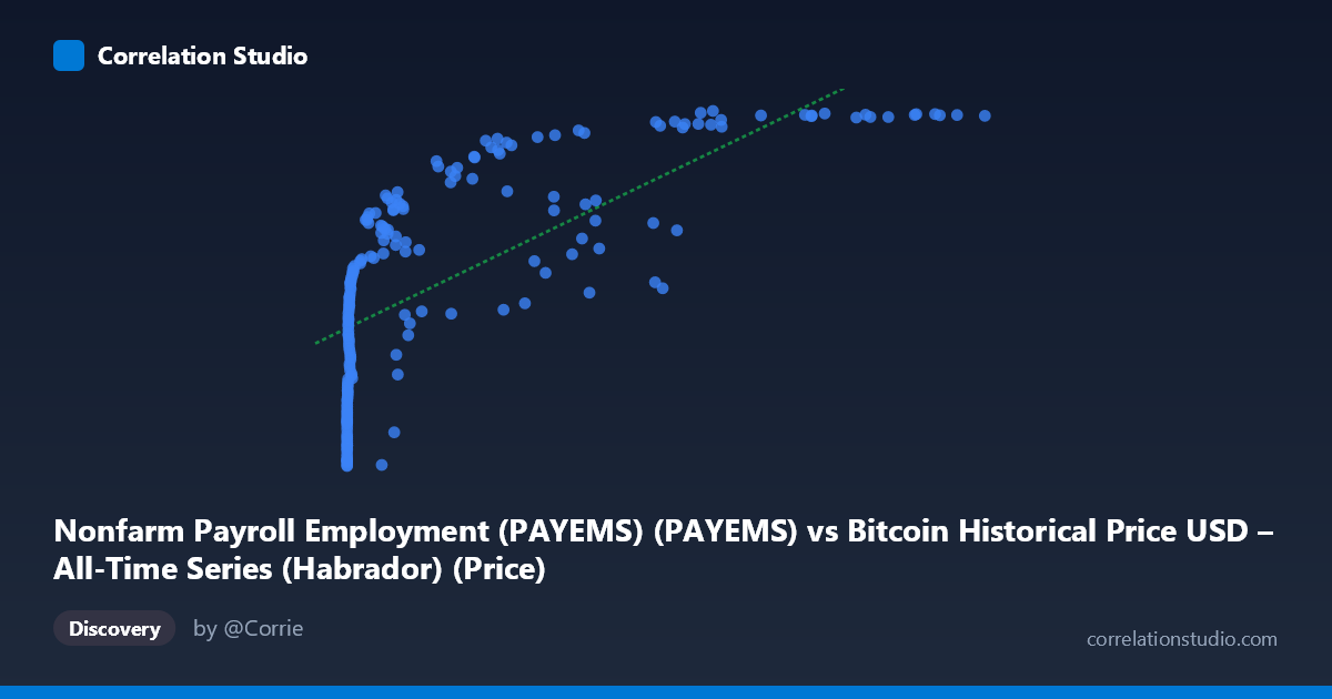
The scatterplot shows a strongly non-linear relationship masquerading as a moderate linear correlation. Bitcoin price (X) spans an enormous range (from $0.06 to $118,670), while Nonfarm Payroll Employment (Y) moves within a comparatively narrow band (130,341 to 158,829 thousand jobs). The data forms a curve reminiscent of a logarithmic or saturating function: at very low Bitcoin prices (under $1,000), employment values are compressed near the low end (~130,000–147,000), but as Bitcoin climbs into the tens of thousands, employment plateaus near its historical ceiling (~156,000–158,800). This pattern is a classic signature of two time series that both trend upward over the same calendar period rather than one directly driving the other.
2. Strength, Direction, and Uncertainty
The Pearson correlation (r = 0.716, r² = 0.513) indicates that a linear model explains about 51% of the variance in employment using Bitcoin price — a moderate-to-strong statistical association, with a tight 95% CI [0.638, 0.779] and p ≈ 0, meaning the correlation itself is not a sampling artifact. However, the note that Spearman's ρ exceeds Pearson's r confirms what the scatter shape suggests: the true relationship is monotonic but non-linear (log-like), so the linear r² likely understates the strength of association once curvature is accounted for. Critically, the Granger causality tests show no significant predictive direction in either direction (X→Y: p=0.417; Y→X: p=0.650) at the optimal lag of 10 periods. This is the most important caveat: despite the strong contemporaneous correlation, neither variable helps forecast the other's future values — the relationship is not causal or lead-lag in nature, but rather a shared-trend coincidence.
3. Notable Patterns and Outliers
Several structural features stand out: - Dense low-X cluster: The majority of sample points cluster at X < 1,000 (Bitcoin's early years), where employment ranges widely (130,000–150,000), reflecting that early Bitcoin price data compresses many different employment states into a narrow X-band — this inflates apparent variance at low X and flattens the curve there. - High-X plateau: Once Bitcoin exceeds ~$40,000–50,000, Y values cluster tightly in the 144,000–158,800 range, with some non-monotonic wobble (e.g., $58,724 → 144,587 vs. $56,973 → 149,816 vs. $60,981 → 157,945) — suggesting employment fluctuations (like COVID-era drops/recoveries) occurred independently of Bitcoin's price trajectory during that window. - Elbow/knee shape: The steepest apparent "rise" in Y happens between X ≈ $300–$30,000, consistent with a log(X) relationship rather than linear.
4. Confounding Factors and Caveats
This is a textbook case of spurious correlation via shared temporal trend. Both series are non-stationary and trending upward over 2010–2026 (Bitcoin due to adoption/speculation cycles; employment due to long-run economic growth with COVID-related disruption). Any two trending time series will show inflated correlation without genuine causal linkage. The Granger non-significance reinforces this: there's no evidence Bitcoin price movements forecast labor market conditions, or vice versa. Additional confounders include: differing native frequencies (Bitcoin trades continuously, PAYEMS is monthly), the extreme scale/skew of Bitcoin prices (log-normal-like distribution) versus the comparatively stable, mildly cyclical employment series, and the fact that macro factors (Fed policy, liquidity, risk sentiment) could jointly influence both without one causing the other.
5. Actionable Insights
For rigorous analysis: (1) detrend or difference both series (e.g., use YoY % changes) before correlating, to test whether the relationship survives removing the shared trend — it likely will not. (2) Fit a log-transformed model (log(X) vs. Y) given the Spearman/Pearson divergence, which should yield a better-fitting, more interpretable functional form. (3) Treat this correlation as descriptive/coincidental for reporting purposes, not predictive or causal — the Granger results should be prominently disclosed to prevent misuse (e.g., claiming "Bitcoin price predicts jobs data" or vice versa). (4) Consider a shared third-factor analysis (e.g., regressing both on time, or on money supply/inflation) to identify the true common driver of their joint upward trends.
X dataset: Bitcoin Historical Price USD – All-Time Series (Habrador)
Y dataset: Nonfarm Payroll Employment (PAYEMS)
Part of experiment: Bitcoin - Bitcoin Historical Price USD – All-Time Series (Habrador) vs Nonfarm Payroll Employment (PAYEMS)