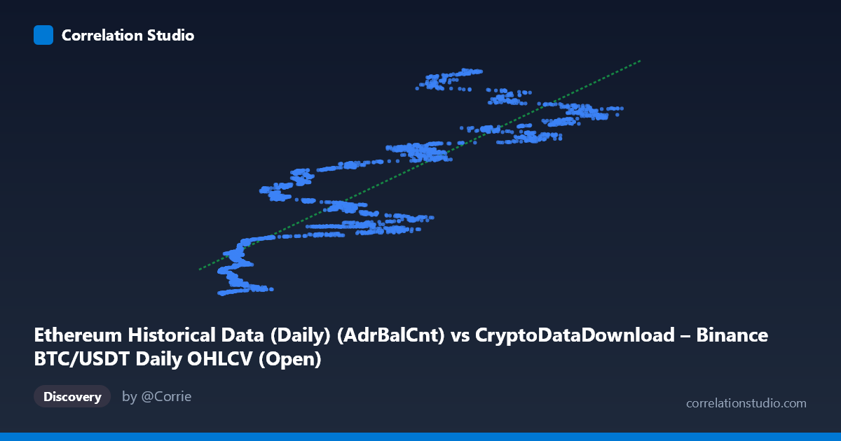
Ethereum Historical Data (Daily) (AdrBalCnt) vs CryptoDataDownload – Binance BTC/USDT Daily OHLCV (Open)
- Pearson correlation (r)
- 0.8575
- Spearman correlation
- 0.8875
- p-value
- 0
- Sample size (n)
- 3191
- 95% confidence interval
- 0.848 to 0.8664
- Granger causality
- None
- Granger optimal lag
- 10
- Time coverage
- 2017-08-17 to 2026-05-20
AI analysis
Analysis of Ethereum Address Count vs. BTC/USDT Open Price
Note on labeling: The axis metadata appears mismatched (X is labeled as an Ethereum on-chain metric, while Y is labeled as a Binance BTC/USDT price column, but the descriptions reference each other's datasets). For this analysis, I'll treat X as the independent variable ("AdrBalCnt"-type network metric) and Y as the dependent price-like variable, as structured in the data.
1. Overall Relationship The scatterplot shows a clear positive, roughly linear relationship between X and Y. As X increases from near-zero values (~3,000–10,000) to higher values (~100,000+), Y climbs from single-digit millions to well over 150 million, with the fitted line (y = 1329.09x + 27.4M) tracking the central tendency of the data reasonably well. The relationship is monotonic and visually tight enough to suggest a genuine shared trend rather than random scatter.
2. Strength, Direction, and Predictive Power The correlation coefficient (r = 0.858) indicates a strong positive linear relationship, and r² = 0.735 tells us that 73.5% of the variance in Y is explained by X — a substantial but not complete explanatory power, leaving roughly 26.5% of variance driven by other factors or noise. The 95% confidence interval [0.848, 0.866] is narrow, and the p-value is effectively 0, meaning this correlation is highly statistically reliable and not a product of sampling error, especially given the large sample size (n=3,191). However, the Granger causality tests show no significant predictive direction in either direction (X→Y: p=0.401; Y→X: p=0.174). This is an important caveat: despite the strong contemporaneous correlation, neither variable reliably predicts future values of the other over a 10-period lag structure. This suggests the relationship may be driven by a shared underlying trend (e.g., both variables growing over the same market cycle) rather than one causally leading the other in time.
3. Patterns, Clusters, and Outliers Several features stand out in the sample data: - Non-uniform variance (heteroscedasticity): At low X values (<15,000), Y is tightly clustered near the regression line’s lower end, but as X grows past 50,000–80,000, the spread in Y widens considerably (e.g., at X≈80,000, Y ranges from ~141M to ~190M). - A possible sub-cluster or inflection region around X = 20,000–35,000, where Y values cluster tightly between 50M–110M, suggesting a possible regime or plateau before the relationship steepens again. - Slight fan/curvature at the upper end, hinting at a possible non-linear (e.g., logarithmic or power-law) relationship rather than strictly linear, common in cumulative network-adoption or price-growth data. - No extreme single-point outliers are obvious, but the variability at high X suggests the linear fit understates uncertainty in that region.
4. Confounding Factors and Caveats Because both variables span a multi-year period (2017–2026) covering multiple crypto market cycles (bull/bear phases), the strong correlation is very likely influenced by a common time trend — both series may simply be growing/declining together due to overall crypto market maturation, adoption, and speculative cycles, rather than a direct causal link between them. Metric mismatches in the axis descriptions also raise data-provenance concerns — confirm the actual variables being compared before drawing further conclusions. Other confounders could include macro liquidity trends, BTC-ETH cross-asset correlation, and network effects that scale together (e.g., more addresses and higher prices both being symptoms of a bull market, not causes of each other).
5. Suggestions for Further Investigation - De-trend both series (e.g., using differencing or detrended residuals) and re-run correlation/Granger tests to check if the relationship holds after removing shared time trends — this is critical given the lack of Granger causality despite high r². - Test non-linear models (log-log or polynomial fits) given the fan-shaped variance at higher X values; a log transformation might better capture the compounding nature of network/price growth. - Segment by market regime (bull vs. bear periods) to see if the relationship strength or slope changes across cycles. - Clarify data provenance to ensure X and Y are correctly labeled, since the current metadata is contradictory and could mislead causal interpretation. - Explore lagged cross-correlations beyond 10 periods, since crypto market dynamics sometimes exhibit longer memory effects than tested here.
X dataset: CryptoDataDownload – Binance BTC/USDT Daily OHLCV
Y dataset: Ethereum Historical Data (Daily)
Part of experiment: Bitcoin - CryptoDataDownload – Binance BTC/USDT Daily OHLCV vs Ethereum Historical Data (Daily)