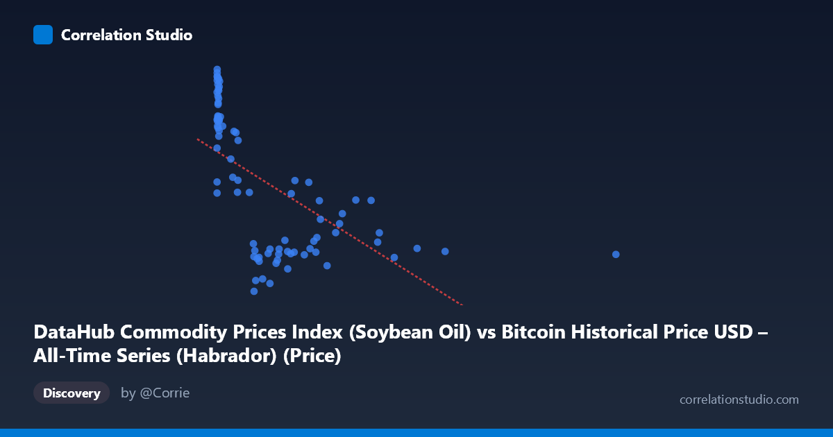
DataHub Commodity Prices Index (Soybean Oil) vs Bitcoin Historical Price USD – All-Time Series (Habrador) (Price)
- Pearson correlation (r)
- -0.5994
- Spearman correlation
- -0.7138
- p-value
- 0
- Sample size (n)
- 83
- 95% confidence interval
- -0.7218 to -0.4406
- Granger causality
- None
- Granger optimal lag
- 10
AI analysis
Analysis of Bitcoin Price vs. Soybean Oil Commodity Index
1. What the Visualization Reveals
The scatterplot shows a moderate negative relationship between the Soybean Oil commodity price index (X) and Bitcoin's historical USD price (Y). The data forms a distinctive pattern: a dense cluster of points at low X-values (roughly 0–50) spans a wide range of Y-values (890–1279), while as X increases beyond ~200, Y values compress into a narrower band (590–930) and gradually decline. This creates a shape resembling a decaying curve rather than a straight line, consistent with the note that Spearman ρ exceeds Pearson r.
2. Strength, Direction, and Statistical Confidence
The Pearson correlation (r = -0.599, r² = 0.359) indicates a moderate negative linear relationship, meaning roughly 36% of the variance in one variable is statistically associated with the other — leaving 64% unexplained, driven by other factors or non-linear dynamics. The 95% CI [-0.722, -0.441] is reasonably tight and entirely negative, and the extremely small p-value (2.14e-09) confirms this relationship is highly unlikely to be due to chance in this sample. However, statistical significance should not be conflated with strong predictive power — with only ~36% shared variance, this is a modest, not dominant, relationship.
Critically, the Granger causality tests show no significant predictive direction: X→Y is clearly non-significant (p=0.375), and Y→X is only marginal (p=0.079, above conventional 0.05 threshold). This means neither variable reliably "leads" or forecasts the other in a time-series sense — the correlation appears to be contemporaneous/structural rather than causal or predictive.
3. Notable Patterns and Non-linear Features
The data clearly follow a curved rather than linear form: a steep drop-off in Y as X rises from 0 to ~250, followed by a long, flat tail where Y stays relatively stable (~700–870) as X extends out to 2452. This logarithmic/power-law shape explains why Spearman's rank correlation is stronger than Pearson's — the relationship is monotonic but not linear. A few high-leverage outliers exist at extreme X values (e.g., X=1402, 2452), which could disproportionately influence the linear regression slope. The tight vertical cluster at very low X (near-zero) with high Y variance (890–1279) suggests another variable is driving Y in that region independent of X.
4. Confounding Factors and Caveats
This pairing is unusual: Bitcoin price is a fast-moving, speculative asset, while the soybean oil index is a traditional commodity indicator — any correlation is likely spurious or mediated by a shared macro factor (e.g., USD strength, global inflation, risk-on/risk-off sentiment, or simply both series trending over the 2010–2017 window due to unrelated secular growth). Since both are time series, non-stationarity (trends within each series) can artificially inflate correlation without true relationship — this is a classic case where correlation ≠ causation, further reinforced by the lack of Granger causality. Additionally, n=83 is a sampled subset of a larger population (N=449), so sampling method and potential autocorrelation in the time series (not independent observations) may bias the r and p-value estimates.
5. Suggested Next Steps
1. Detrend or difference both series (e.g., use returns/percent changes instead of levels) and re-test correlation and Granger causality to rule out spurious trend-driven correlation. 2. Fit a non-linear model (log-log, power law, or polynomial) given the curved pattern and Spearman/Pearson discrepancy — this will likely explain more variance than the linear r²=0.36. 3. Test for a common confounding variable (e.g., USD index, inflation, or overall market liquidity) that may independently drive both series. 4. Check stationarity (ADF test) before trusting Granger causality results, as non-stationary series can produce unreliable causality tests. 5. Treat this relationship as descriptive/associative only — it should not be used for trading or forecasting one variable from the other given the absence of causal evidence.
X dataset: Bitcoin Historical Price USD – All-Time Series (Habrador)
Y dataset: DataHub Commodity Prices Index
Part of experiment: Bitcoin - Bitcoin Historical Price USD – All-Time Series (Habrador) vs DataHub Commodity Prices Index