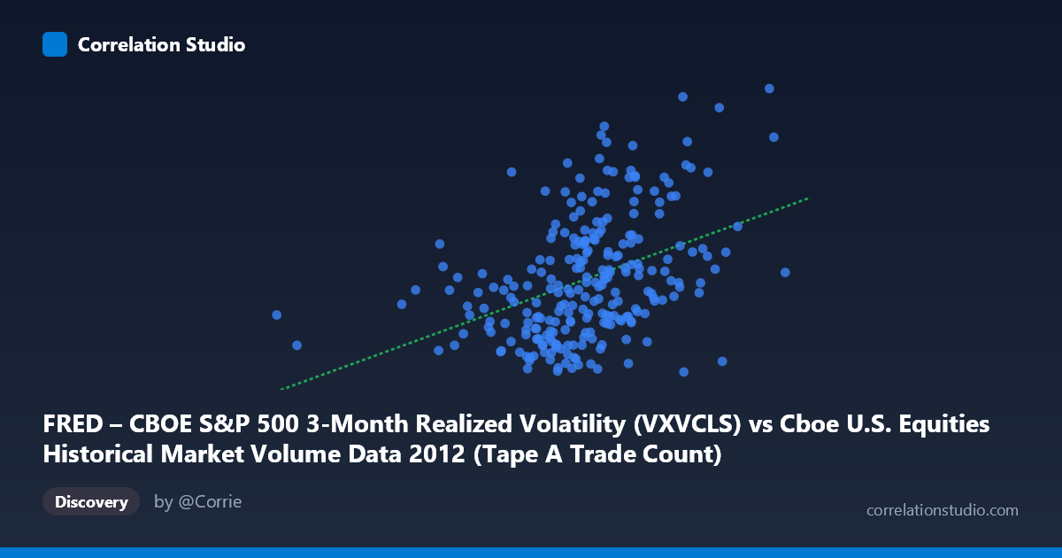
FRED – CBOE S&P 500 3-Month Realized Volatility (VXVCLS) vs Cboe U.S. Equities Historical Market Volume Data 2012 (Tape A Trade Count)
- Pearson correlation (r)
- 0.411
- Spearman correlation
- 0.436
- p-value
- 0
- Sample size (n)
- 250
- 95% confidence interval
- 0.3023 to 0.5091
- Granger causality
- None
- Granger optimal lag
- 1
AI analysis
Analysis: CBOE S&P 500 3-Month Realized Volatility vs. Tape A Trade Count (2012)
Relationship Overview
The scatterplot reveals a modest positive relationship between CBOE S&P 500 3-month realized volatility (VXVCLS) and Tape A trade counts across U.S. equity exchanges during 2012. As volatility increases, trade counts tend to rise alongside it — a directionally intuitive finding, since elevated market uncertainty typically drives greater trading activity as participants reposition, hedge, or react to price dislocations. The linear regression equation (y = 7.30×10⁻⁶x + 13.07) confirms this upward slope, though the scatter around the regression line is visibly wide, signaling that the relationship is far from deterministic.
Correlation Strength and Statistical Significance
The correlation of r = 0.411 represents a moderate positive association, but the explanatory power is limited: r² = 0.169 means only about 16.9% of the variance in trade counts is explained by volatility levels, leaving roughly 83% attributable to other factors. The 95% confidence interval of [0.30, 0.51] is reasonably tight and does not cross zero, and the p-value of 1.31×10⁻¹¹ confirms the relationship is highly statistically significant — effectively ruling out chance given n = 250 paired observations. However, statistical significance here is largely a function of sample size and should not be conflated with practical or economic significance. Critically, Granger causality tests find no significant predictive directionality in either direction (X→Y: F = 0.587, p = 0.444; Y→X: F = 0.615, p = 0.434), meaning that past volatility readings do not meaningfully predict future trade counts, and vice versa, at the tested lag of one period. This suggests the observed correlation reflects contemporaneous co-movement rather than any exploitable lead-lag or causal mechanism.
Notable Patterns, Clusters, and Outliers
Several features stand out in the scatterplot. The bulk of observations cluster in a mid-range band — roughly X values between 850,000 and 1,200,000 with Y values between 17 and 23 — forming a dense core where the positive trend is most evident. However, there are notable high-Y outliers (trade counts reaching 25–28, visible in points like (1,031,530, 25.50), (1,035,061, 26.50), (1,046,601, 26.19), and (964,117, 25.31)) that sit well above the regression line, suggesting episodes where volatility spiked independently of volume patterns. Conversely, there are low-X, low-Y observations at the left tail (e.g., X ~732,000–800,000 with Y ~18–20) that hint at quieter market regimes. The wide vertical dispersion at any given X value reinforces that a single volatility reading offers limited precision in predicting trade counts on any given day.
Confounding Factors and Interpretive Caveats
Several important caveats apply. First, the axes appear swapped relative to conventional labeling — the X-axis is described as the VXVCLS volatility index yet the range (350,659–1,423,452) matches a trade count scale, while the Y-axis range (16–28) matches a volatility index. This likely reflects a dataset column assignment reversal, and the substantive interpretation should be verified against the raw data. Second, seasonality and macro events in 2012 (e.g., the European debt crisis, U.S. election, fiscal cliff fears) could drive simultaneous spikes in both volatility and trading volume, creating spurious or inflated correlations. Third, structural market factors — algorithmic trading patterns, options expiration cycles, and exchange-specific rule changes — independently affect Tape A trade counts regardless of volatility. Finally, the data covers only a single calendar year (2012), limiting generalizability across different market regimes.
Actionable Insights and Further Investigation
Given the moderate but incomplete correlation and absence of Granger causality, practitioners should avoid using lagged volatility as a standalone predictor of daily trade volume for operational or strategic planning purposes. A more productive path would involve: (1) expanding the time series across multiple years and market regimes to test whether the r ≈ 0.41 relationship is stable or regime-dependent; (2) introducing additional covariates such as VIX level, bid-ask spreads, or macroeconomic event indicators to build a more complete model of trade count drivers; (3) testing non-linear specifications (e.g., threshold or regime-switching models) given the visible heteroscedasticity in the scatterplot; and (4) resolving the axis ambiguity in the dataset column assignments before drawing firm conclusions. The contemporaneous nature of the correlation also suggests that intraday or higher-frequency analysis might reveal tighter, more actionable relationships between volatility and trading activity than daily aggregates permit.
X dataset: Cboe U.S. Equities Historical Market Volume Data 2012
Y dataset: FRED – CBOE S&P 500 3-Month Realized Volatility
Part of experiment: Daily - Cboe U.S. Equities Historical Market Volume Data 2012 vs FRED – CBOE S&P 500 3-Month Realized Volatility