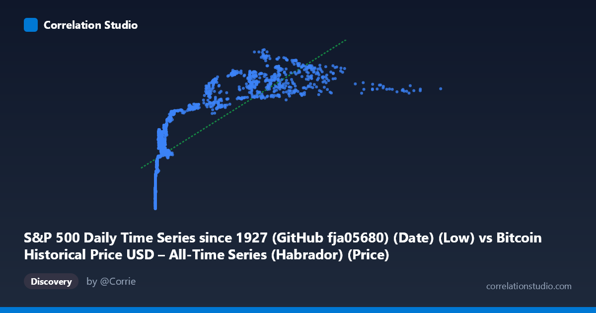
S&P 500 Daily Time Series since 1927 (GitHub fja05680) (Date) (Low) vs Bitcoin Historical Price USD – All-Time Series (Habrador) (Price)
- Pearson correlation (r)
- 0.7838
- Spearman correlation
- 0.9423
- p-value
- 0
- Sample size (n)
- 2376
- 95% confidence interval
- 0.7678 to 0.7989
- Granger causality
- X → Y
- Granger optimal lag
- 1
AI analysis
Analysis: Bitcoin Price vs. S&P 500 Price Relationship
Note on labeling: The axis labels appear swapped in the metadata (X described as S&P 500, Y as Bitcoin), but the data values themselves (X ranging to 18,960 with heavy right-skew; Y bounded between ~1,040–3,222) clearly indicate X = Bitcoin price and Y = S&P 500 price. This analysis proceeds on that basis.
1. What the Visualization Reveals
The scatterplot shows a curved, monotonically increasing relationship between Bitcoin price (X) and the S&P 500 (Y). At low Bitcoin values (under $1,000), the S&P 500 spans a wide range (roughly 1,300–2,300), producing a dense, near-vertical cluster of points. As Bitcoin climbs into the thousands and eventually above $10,000, the S&P 500 values compress into a narrower, higher band (2,700–3,200). This produces a classic logarithmic or square-root shaped curve rather than a straight line — consistent with the note that Spearman's ρ exceeds Pearson's r.
2. Strength, Direction, and Uncertainty
The linear Pearson correlation (r = 0.784) indicates a strong positive association, with r² = 0.614 meaning the linear model explains about 61% of the variance in S&P 500 levels using Bitcoin price alone. The 95% CI [0.768, 0.799] is tight, and the p-value is effectively zero, so the correlation itself is highly statistically reliable — not a chance artifact of sampling. However, statistical significance here reflects the enormous sample size and shared trending behavior over time, not necessarily a meaningful causal economic relationship. The Granger causality test found that Bitcoin price changes help predict future S&P 500 movements (F = 6.41, p = 0.011) at a 1-period lag, while the reverse (S&P 500 → Bitcoin) is not significant (p = 0.091). This is a weak, marginal directional signal at best, and should not be over-interpreted as genuine economic causality — more likely both series are driven by a shared underlying time trend.
3. Notable Patterns and Non-linearity
The most striking feature is the compression/saturation pattern: enormous swings in Bitcoin price (from cents to tens of thousands of dollars) correspond to comparatively modest, bounded movements in the S&P 500 (roughly 1,000–3,200). This is characteristic of comparing an asset with multiple orders-of-magnitude growth (Bitcoin, log-scale behavior) against one with steady, bounded appreciation (S&P 500, roughly linear/exponential but far gentler). A log-transform of X would likely straighten the relationship substantially and improve fit — consistent with the Spearman Pearson observation. There's also a visible dense cluster at low X values (sub-$1,000 Bitcoin) mapping to S&P 500 values spanning nearly the entire observed range, indicating high variance in Y is concentrated in Bitcoin's early history.
4. Confounding Factors and Caveats
This is almost certainly a spurious/trend-driven correlation rather than a direct causal or fundamental economic linkage. Both Bitcoin and the S&P 500 have exhibited long-term upward trends over the 2010–2019 window (Bitcoin due to adoption/speculation growth from near-zero; S&P 500 due to the post-financial-crisis bull market). Any two non-stationary time series trending upward over the same period will show strong correlation without genuine causal linkage — this is a well-known pitfall (spurious regression) in time-series analysis. The data are not de-trended, differenced, or tested for stationarity/cointegration, so the correlation coefficient and Granger test results are likely confounded by shared calendar-time trends rather than true interdependence. Additionally, pairing "Bitcoin price on date D" with "S&P 500 price on date D" via merged datasets can introduce alignment artifacts (e.g., weekends/holidays when one market is closed).
5. Suggestions for Further Investigation
- Detrend/difference the data: Analyze daily/weekly returns (percentage changes) rather than price levels, and re-test correlation and Granger causality — this is the standard fix for spurious trend correlation. - Log-transform Bitcoin price: Given its exponential growth, refit the regression as Y ~ log(X) or Y ~ X^0.5 to test whether it improves R² materially over the linear fit. - Cointegration testing: Run an Engle-Granger or Johansen cointegration test to assess whether a genuine long-run equilibrium relationship exists beyond shared trending. - Segment by time period: Since Time coverage spans 2010–2019, check whether the correlation holds within sub-periods (e.g., 2010-2014 vs. 2015-2019) or is driven by a few high-growth episodes (like Bitcoin's 2017 rally). - Treat Granger result cautiously: Given the marginal p-value (0.011, not overwhelming) and known confounding, do not use this as a basis for trading strategies without stationarity-corrected reanalysis.
X dataset: Bitcoin Historical Price USD – All-Time Series (Habrador)
Y dataset: S&P 500 Daily Time Series since 1927 (GitHub fja05680) (Date)
Part of experiment: Bitcoin - Bitcoin Historical Price USD – All-Time Series (Habrador) vs S&P 500 Daily Time Series since 1927 (GitHub fja05680) (Date)