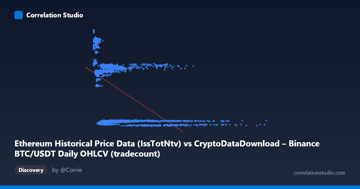
Ethereum Historical Price Data (IssTotNtv) vs CryptoDataDownload – Binance BTC/USDT Daily OHLCV (tradecount)
- Pearson correlation (r)
- -0.5339
- Spearman correlation
- -0.5516
- p-value
- 0
- Sample size (n)
- 3191
- 95% confidence interval
- -0.5583 to -0.5087
- Granger causality
- None
- Granger optimal lag
- 10
- Time coverage
- 2017-08-17 to 2026-05-20
AI analysis
Scatterplot Analysis: X (IssTotNtv) vs Y (tradecount)
1. Overall Relationship The visualization shows a moderate negative, distinctly non-linear relationship between the two variables. Rather than a smooth downward slope, the data appear to cluster into distinct horizontal bands (roughly around y≈2,000-2,800, y≈13,400-14,900, and y≈20,000-21,000), with X values decreasing as Y-band increases. This banding pattern suggests the underlying data may represent discrete regimes or categories rather than a continuous functional relationship — possibly different time periods, market phases, or measurement contexts collapsed onto this single scatter.
2. Strength, Direction, and Statistical Confidence The correlation coefficient (r = -0.534, R² = 0.285) indicates a moderate negative association, but one that leaves 71.5% of Y's variance unexplained — meaning X alone is a weak predictor of Y in practical terms. The confidence interval [-0.558, -0.509] is tight and excludes zero, and the p-value is effectively 0, confirming the correlation is statistically robust and not due to chance given the large sample (n=3,191). However, statistical significance here reflects sample size more than practical predictive strength — R² of 0.285 means the linear model explains only about a quarter to a third of the pattern seen.
Critically, the Granger causality tests show no significant predictive direction in either direction (X→Y: p=0.172; Y→X: p=0.241). This is an important caveat: despite the correlation, neither variable helps forecast the other's future values based on past values at the tested lag (10 periods). This suggests the correlation is likely contemporaneous/structural rather than causal or dynamically predictive — both variables may be co-moving due to shared external drivers (e.g., overall market conditions, time trends) rather than one driving the other.
3. Notable Patterns and Outliers The most striking feature is the multi-modal clustering in Y — three or four distinct horizontal strata are visible rather than a continuous cloud. Within each band, X spans a wide range (from near-zero to over 8 million), but higher Y-bands are almost exclusively associated with low X values (under ~1 million), while the low-Y band (~2,000-2,800) contains the highest X values (up to 15+ million). This looks like a threshold or saturation effect: once X exceeds roughly 1-2 million, Y collapses into the lowest band, while small X values permit a wide range of Y outcomes. A few extreme X outliers (8 million) sit at the low end of Y, potentially exerting heavy leverage on the linear regression slope.
4. Confounding Factors and Caveats Several caveats are important: - Time confounding: Both series span 2017-2026, a period of major structural change in crypto markets (bull/bear cycles, exchange volume shifts, network upgrades like Ethereum's PoS transition). Both variables may simply trend with calendar time rather than with each other directly. - Mismatched metrics: X is derived from Ethereum issuance/native units while Y is Binance BTC/USDT tradecount — these come from different assets and dataset labels are inconsistently described, raising concern about data alignment/joining errors (e.g., joined on date without accounting for asset differences). - Non-linearity: Given the banded/threshold pattern, Pearson's r and linear R² understate or mischaracterize the true relationship; a linear model is a poor fit here. - Outlier leverage: A handful of very large X values could be distorting both the correlation estimate and regression slope.
5. Recommendations Given the ambiguous variable labeling (Ethereum column feeding an "X-axis" tied to BTC/USDT dataset naming), first verify data provenance and join logic — this may be a data pipeline artifact rather than a genuine economic relationship. Next, investigate the banding structure directly: segment the data by time period or by the apparent Y-clusters and check whether each cluster corresponds to a distinct market regime (e.g., specific years or volatility regimes). A non-linear or regime-switching model (e.g., piecewise regression, quantile regression, or clustering analysis) would likely reveal more than the linear fit. Finally, given the null Granger result, avoid using this relationship for forecasting; instead, treat it as evidence of shared time-trend or regime co-movement, and consider testing both series against a common third variable (e.g., overall market cap, date, or volatility index) to identify the true underlying driver.
X dataset: CryptoDataDownload – Binance BTC/USDT Daily OHLCV
Y dataset: Ethereum Historical Price Data
Part of experiment: Bitcoin - CryptoDataDownload – Binance BTC/USDT Daily OHLCV vs Ethereum Historical Price Data