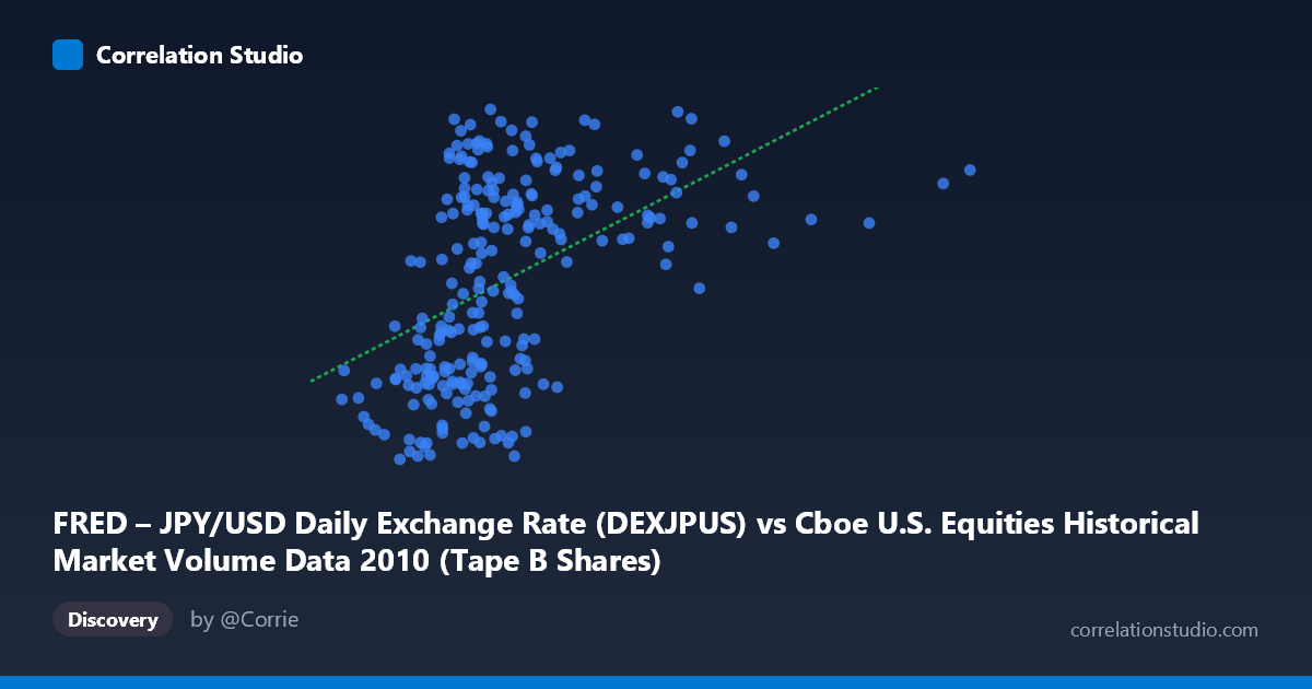
FRED – JPY/USD Daily Exchange Rate (DEXJPUS) vs Cboe U.S. Equities Historical Market Volume Data 2010 (Tape B Shares)
- Pearson correlation (r)
- 0.4831
- Spearman correlation
- 0.5287
- p-value
- 0
- Sample size (n)
- 249
- 95% confidence interval
- 0.3818 to 0.573
- Granger causality
- None
- Granger optimal lag
- 1
AI analysis
Analysis: JPY/USD Exchange Rate vs. Cboe Tape B Share Volume (2010)
Relationship Overview The scatterplot reveals a moderate positive relationship between U.S. equity market volume (Tape B shares, on the X-axis) and the JPY/USD exchange rate (Y-axis) across 249 trading days in 2010. As daily Tape B share volume increases, the yen tends to appreciate against the dollar (higher JPY/USD values mean more yen per dollar, indicating dollar strength — or conversely, the rate reflects the prevailing exchange environment). The linear regression equation y = 4.54×10⁻⁸x + 82.59 suggests that each additional ~22 million shares traded corresponds to roughly a one-unit increase in the exchange rate, though the scatter around this line is considerable. The relationship is positive but far from deterministic, with a wide spread of Y values across nearly the full X range.
Correlation Strength and Statistical Significance The Pearson correlation of r = 0.483 indicates a moderate positive association, but the more informative metric is r² = 0.233, meaning that only about 23.3% of the variance in the JPY/USD rate is explained by Tape B share volume. This leaves over 76% of variation attributable to other factors entirely. The 95% confidence interval of [0.38, 0.57] is reasonably tight given n = 249, and the p-value of 6.66×10⁻¹⁶ confirms the correlation is highly statistically significant — effectively ruling out a chance finding. However, statistical significance here is partly a function of the large population (N = 3,302) and should not be conflated with practical or economic significance. Critically, Granger causality tests show no significant predictive directionality in either direction (X→Y: F = 0.32, p = 0.57; Y→X: F = 0.16, p = 0.69), meaning neither variable reliably predicts the future values of the other at a one-period lag. This strongly cautions against any causal or forecasting interpretation of the correlation.
Patterns, Clusters, and Outliers The scatterplot exhibits notable structural features worth examining. There appear to be two loose clusters: one concentrated in the lower-volume, lower-rate region (roughly X < 100M shares, Y between 80–86), and another in the moderate-to-high volume range (100–200M shares) with exchange rates spanning 87–94. A vertical band effect is visible — at similar volume levels, the exchange rate varies by as much as 10–12 points, suggesting high conditional variance. Several potential outliers stand out, including points near X ≈ 37.5M (minimum volume, Y ≈ 82.9) and X ≈ 328M (maximum volume), as well as high-Y observations above 93–94 at moderate volume levels (~97–125M shares). The distribution along the X-axis is right-skewed, with most observations clustered below 150M shares and a long tail extending toward 330M, which may be influencing the regression slope.
Confounding Factors and Interpretive Caveats This correlation almost certainly reflects shared temporal confounding rather than a direct economic mechanism. Both equity market volume and JPY/USD exchange rates are influenced by broad macroeconomic forces — risk sentiment, Federal Reserve policy, global capital flows, and geopolitical events — that evolve together over 2010. The post-financial-crisis recovery period featured distinct regime shifts (e.g., QE announcements, European debt crisis episodes) that could simultaneously drive both variables upward or downward, generating spurious correlation. The note-worthy label swap in the dataset metadata (X-axis is labeled as JPY/USD but described as "market volume," and Y-axis vice versa) warrants careful verification before drawing any conclusions. Additionally, Tape B shares represent only a subset of U.S. equity market activity, and using a single-lag Granger test may be insufficient to capture more complex delayed dynamics.
Actionable Insights and Further Investigation Given the moderate but unexplained variance and absence of Granger causality, practitioners should avoid using equity volume as a direct predictor of JPY/USD rates or vice versa. A more productive investigation would involve: (1) controlling for known macro drivers such as VIX, U.S. Treasury yields, or Fed announcement dates to test whether the correlation persists; (2) extending the Granger analysis to multiple lags (e.g., 2–5 periods) to rule out longer-horizon predictive relationships; (3) segmenting the data by market regime or quarter to test whether the correlation is stable or driven by a specific sub-period in 2010; and (4) verifying axis labeling in the source data to ensure the variable assignments are correct. If the correlation proves robust after controls, it may reflect meaningful risk-on/risk-off dynamics linking currency markets and equity trading activity — a hypothesis worth testing with a broader multi-year dataset.
X dataset: Cboe U.S. Equities Historical Market Volume Data 2010
Y dataset: FRED – JPY/USD Daily Exchange Rate
Part of experiment: Daily - Cboe U.S. Equities Historical Market Volume Data 2010 vs FRED – JPY/USD Daily Exchange Rate