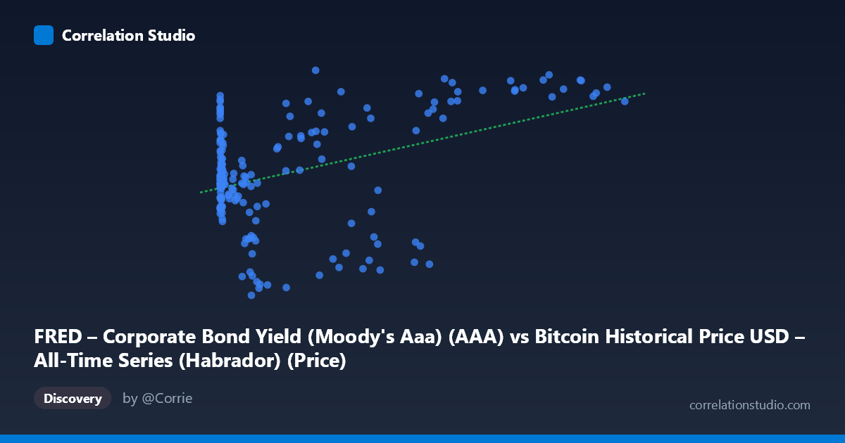
FRED – Corporate Bond Yield (Moody's Aaa) (AAA) vs Bitcoin Historical Price USD – All-Time Series (Habrador) (Price)
- Pearson correlation (r)
- 0.4176
- Spearman correlation
- 0.157
- p-value
- 0
- Sample size (n)
- 189
- 95% confidence interval
- 0.2923 to 0.5288
- Granger causality
- None
- Granger optimal lag
- 1
AI analysis
Analysis: Bitcoin Price vs. Corporate Bond Yield (Moody's Aaa)
1. What the Visualization Reveals
The scatterplot shows a weak-to-moderate positive relationship between Bitcoin's historical price (X-axis) and Moody's Aaa corporate bond yield (Y-axis). At low Bitcoin prices (under $1,000), bond yields scatter broadly between roughly 3.5% and 5.0%, showing no clear pattern. As Bitcoin prices climb into the tens of thousands, yields trend somewhat higher on average, but with substantial scatter — including several notable low-yield readings (2.3–3.0%) at high Bitcoin prices ($13,000–$58,000 range). The relationship is far from a clean linear trend; it looks more like a loose, noisy upward drift with significant dispersion at every price level.
2. Strength, Direction, and Statistical Interpretation
The correlation coefficient (r = 0.418) indicates a modest positive association, but r² = 0.174 means only 17.4% of the variance in bond yields is explained by Bitcoin price (or vice versa) — leaving over 82% unexplained by this simple linear relationship. The 95% confidence interval [0.292, 0.529] is reasonably tight and excludes zero, and the p-value (2.26E-09) confirms this correlation is highly unlikely to be due to chance in this sample. However, statistical significance here reflects sample size and consistency, not practical strength — this is a weak-to-moderate relationship, not one suitable for precise prediction.
Critically, the Granger causality tests show no significant predictive direction in either direction (Bitcoin→Yield: p=0.68; Yield→Bitcoin: p=0.80). This means neither variable's past values help forecast the other's future values in a time-series sense. Combined with the low r², this strongly suggests the correlation is likely driven by a shared underlying trend (e.g., both series broadly rising over the 2010–2026 period, or both responding to a common macro regime) rather than any causal or lead-lag mechanism connecting them directly.
3. Notable Patterns and Outliers
Several features stand out: - Non-stationarity artifact: Bitcoin price grew exponentially over this period (from cents to over $100,000), while bond yields fluctuated in a bounded range (2.14–5.61%). Correlating a near-exponential trend with a bounded oscillating series can produce spurious positive correlation purely from co-occurring long-term drift. - Low-yield cluster at high prices: Points like (41,869, 2.55), (34,856, 2.57), (13,891, 2.30) show that some of the highest Bitcoin prices coincided with historically low bond yields — likely the 2020–2021 near-zero-rate era, contradicting a simple positive linear story. - High-yield cluster at high prices: Conversely, points like (105,620, 5.46), (96,467, 5.54) show recent high Bitcoin prices coinciding with elevated yields (the 2023–2024 rate-hiking cycle). - These two clusters suggest the relationship may be regime-dependent rather than continuously linear — different macro eras (ZIRP vs. post-2022 tightening) dominate different segments of the Bitcoin price range.
4. Confounding Factors and Caveats
This correlation is very likely confounded by time itself. Both Bitcoin price and bond yields are non-stationary time series with strong secular trends (Bitcoin's adoption-driven exponential growth; bond yields' multi-year cycles tied to Fed policy). Any two trending series measured over the same calendar period can show spurious correlation without genuine economic linkage. Additional confounders include: macroeconomic regime shifts (2020 pandemic near-zero rates vs. 2022+ tightening), the highly skewed distribution of Bitcoin prices (mean $20,533 vs. median far lower, given the range extends to $118,670), and potential non-linearity poorly captured by a linear model (r² of only 17%).
5. Suggestions for Further Investigation
- De-trend both series (e.g., use log returns or first differences instead of levels) before correlating, to remove spurious trend-driven correlation and test whether a genuine relationship survives. - Segment by macro regime (pre-2020, 2020–2021 ZIRP, 2022+ tightening) to check if the relationship sign/strength changes across periods — the clusters noted above suggest it might. - Test alternative explanatory variables — real interest rates, inflation expectations, or risk-asset sentiment indices (e.g., S&P 500, VIX) may better explain Bitcoin price movements than nominal Aaa yields alone. - Given the null Granger causality result, avoid using one series to forecast the other; instead, treat any correlation as descriptive/coincidental rather than predictive for trading or policy purposes.
X dataset: Bitcoin Historical Price USD – All-Time Series (Habrador)
Y dataset: FRED – Corporate Bond Yield (Moody's Aaa)
Part of experiment: Bitcoin - Bitcoin Historical Price USD – All-Time Series (Habrador) vs FRED – Corporate Bond Yield (Moody's Aaa)