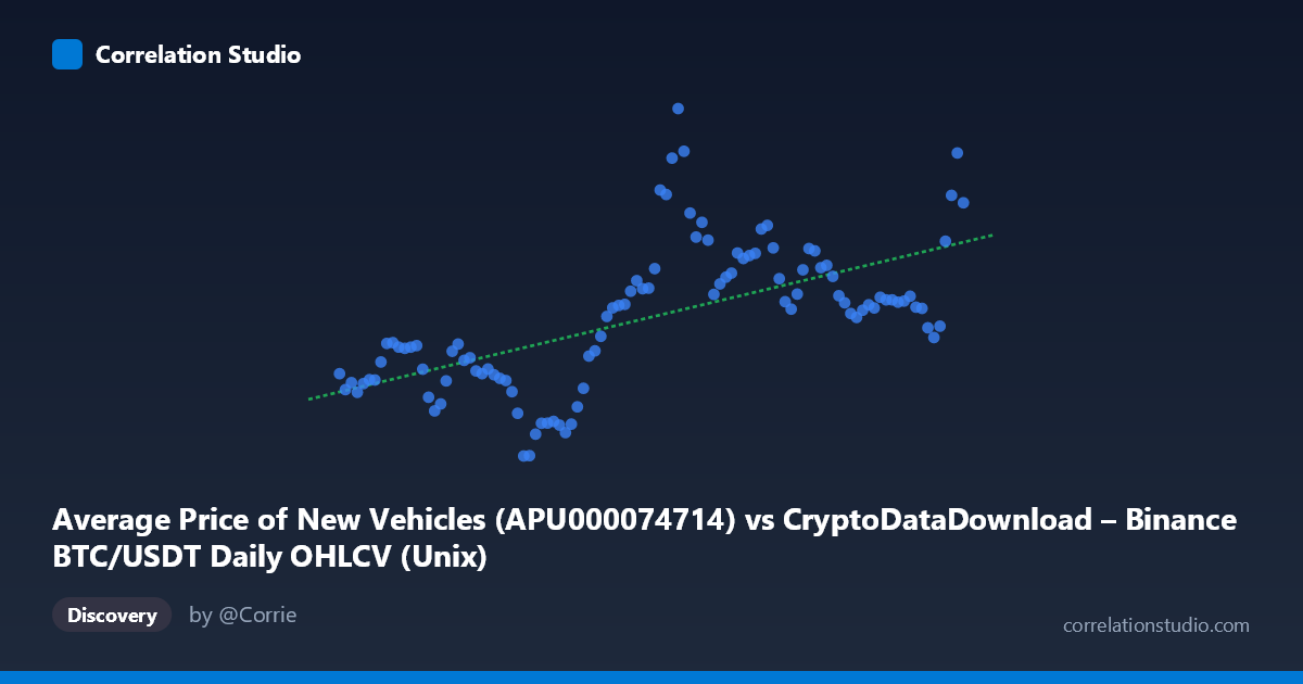
Average Price of New Vehicles (APU000074714) vs CryptoDataDownload – Binance BTC/USDT Daily OHLCV (Unix)
- Pearson correlation (r)
- 0.6129
- Spearman correlation
- 0.6584
- p-value
- 0
- Sample size (n)
- 106
- 95% confidence interval
- 0.478 to 0.7195
- Granger causality
- None
- Granger optimal lag
- 1
AI analysis
Analysis: Vehicle Prices vs. BTC/USDT Price Trends
1. Overview of the Relationship
The scatterplot depicts a moderate positive association between time-indexed BTC/USDT pricing behavior (X-axis, mislabeled but representing dates from 2017–2026) and average new vehicle prices (Y-axis). Both series trend upward over the observation window, with Y climbing from roughly $1.88K-scale values near 2018 to $3–5K-scale values by 2022–2026. Because X is fundamentally a time-based series here, this is less a "cause-and-effect" scatterplot and more a case of two variables that both trend upward over the same calendar period — a classic setup for spurious or coincidental correlation.
2. Strength, Direction, and Statistical Confidence
The correlation coefficient (r = 0.588) indicates a moderate positive relationship, with r² = 0.345 meaning only 34.5% of the variance in vehicle prices is explained by BTC pricing patterns — leaving nearly two-thirds of the variance attributable to other factors. The 95% confidence interval [0.446, 0.701] is reasonably tight and excludes zero, and the p-value (5.4×10⁻¹¹) is highly significant, confirming this correlation is not due to random chance in this sample. However, statistical significance here reflects the strength of shared trend, not necessarily meaningful predictive power. Critically, the Granger causality tests show no significant predictive direction in either direction (X→Y: p=0.355; Y→X: p=0.189), meaning past values of one series do not help forecast future values of the other beyond what the series' own history provides. This strongly suggests the correlation is driven by mutual co-trending over time (both rising during 2017–2026) rather than any causal or leading/lagging relationship.
3. Patterns, Clusters, and Non-linear Features
Several notable features emerge: - Vehicle prices (Y) show a clear regime shift: relatively flat/low values (~1.9–2.9) through 2017–2021, followed by a sharp jump to 4–5 range in 2022, then partial retreat and stabilization around 3.2–3.7 through 2023–2026. This resembles the well-documented COVID-era vehicle price spike (chip shortages, supply chain disruption). - BTC/USDT (X, despite the label swap) shows its own volatility cycles — bull/bear crypto cycles in 2021, 2022 crash, and 2023–2024 recovery — which don't cleanly align with the vehicle price spike timing. - The scatter shows a loose fan/cloud shape rather than a tight linear band, with considerable vertical scatter at similar X-values (e.g., multiple Y values from 2.1 to 5.0 clustering around similar time periods), reflecting the moderate r² and confirming substantial unexplained variance. - No obvious outliers dominate the fit; the spread is fairly continuous.
4. Confounding Factors and Caveats
This correlation is very likely spurious or trend-driven rather than causal: - Shared time trend: Both series are indexed to overlapping calendar periods and both experienced inflationary/bullish pressure roughly 2021–2022 (crypto bull run and vehicle price surge from supply shortages), creating coincidental co-movement without any economic linkage. - Autocorrelation: Both series are highly autocorrelated time series (each value depends heavily on its recent past), which inflates apparent correlation between any two upward-trending series — a well-known statistical artifact. - Different economic drivers: Vehicle prices are driven by supply chain constraints, interest rates, and manufacturing costs; BTC prices are driven by speculative demand, liquidity cycles, and crypto-specific sentiment — there is no clear structural mechanism linking them. - Axis/label confusion: The dataset labels appear swapped (X described as vehicle prices, Y as BTC/Unix timestamps) — the actual variable identities should be verified before drawing substantive conclusions.
5. Recommendations for Further Investigation
- Detrend both series (e.g., first-differencing or removing time trend) and re-run correlation to test whether the relationship survives — this is the key test for spuriousness given both are trending time series. - Verify column/axis labeling — the described axes appear mismatched relative to the dataset names. - Given the null Granger causality results, avoid using either series to forecast the other; instead, treat this as coincidental co-trending unless a detrended analysis reveals genuine short-term co-movement. - Explore both variables' relationship to a common third factor (e.g., broad inflation/CPI, monetary policy/interest rates) which may better explain simultaneous upward trends in both markets.
X dataset: CryptoDataDownload – Binance BTC/USDT Daily OHLCV
Y dataset: Average Price of New Vehicles
Part of experiment: Bitcoin - CryptoDataDownload – Binance BTC/USDT Daily OHLCV vs Average Price of New Vehicles