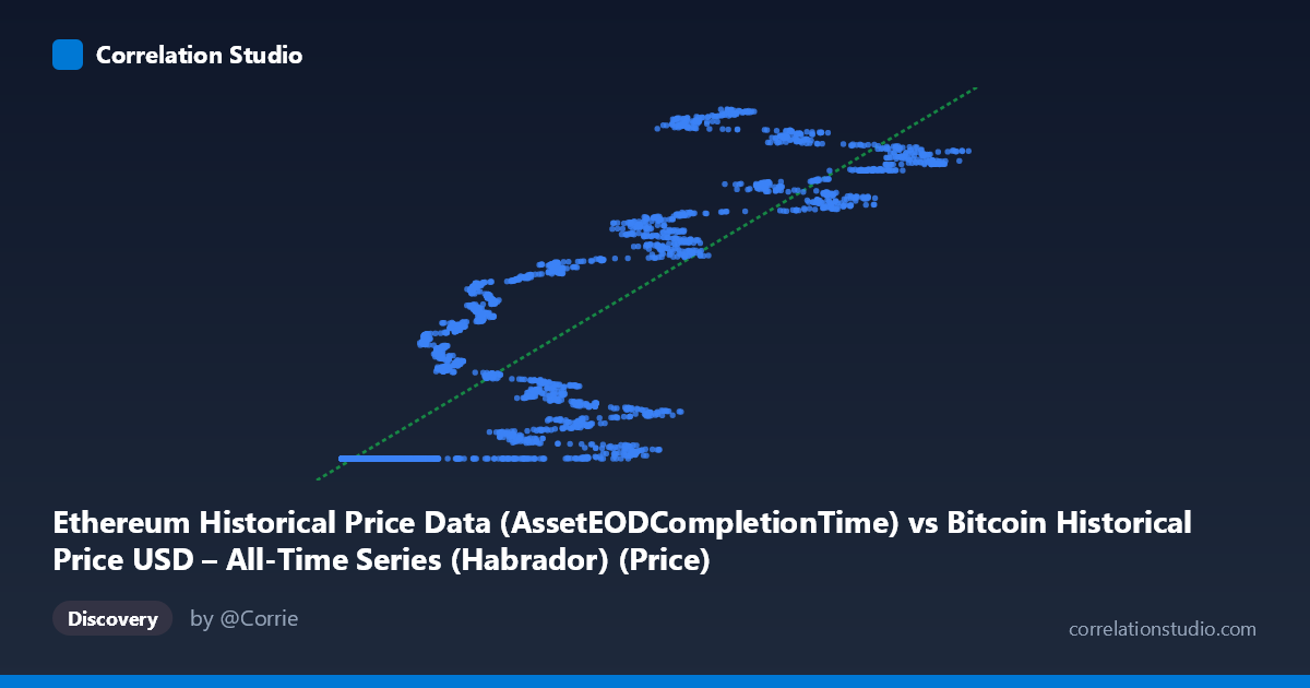
Ethereum Historical Price Data (AssetEODCompletionTime) vs Bitcoin Historical Price USD – All-Time Series (Habrador) (Price)
- Pearson correlation (r)
- 0.8733
- Spearman correlation
- 0.9402
- p-value
- 0
- Sample size (n)
- 3951
- 95% confidence interval
- 0.8657 to 0.8805
- Granger causality
- None
- Granger optimal lag
- 10
- Time coverage
- 2015-07-30 to 2026-05-23
- Recomputed on refreshed data
- 2026-10-24 (r was 0.8726)
AI analysis
Analysis: Ethereum Price vs. Bitcoin Price Relationship
1. Overview of the Relationship
Despite the column labels being somewhat crossed in the metadata (X is described as Ethereum-related, Y as Bitcoin-related), the underlying data clearly represents two major cryptocurrency price series plotted against each other. The scatterplot reveals a strong positive, non-linear relationship: as the X variable increases, Y increases as well, but the relationship shows clear saturation/plateau behavior at the low end and steep escalation at the high end, rather than a clean straight line.
2. Strength, Direction, and Statistical Confidence
The correlation coefficient (r = 0.8726, r² = 0.7615) indicates a strong positive linear association, with approximately 76% of the variance in Y statistically explained by X — a substantial but not complete relationship, leaving ~24% of variance driven by other factors or non-linear dynamics. The 95% CI [0.8650, 0.8799] is tight, reflecting the large sample size (n=3,926) and giving high confidence that the true population correlation sits in this narrow band. The p-value of 0 (effectively <0.0001) confirms this correlation is not due to chance.
However, the Granger causality tests are critical for tempering interpretation: neither variable significantly predicts the other in a temporal/lagged sense (X→Y: p=0.9618; Y→X: p=0.7187, at 10 lags). This means despite the strong contemporaneous correlation, there is no statistical evidence that movements in one series lead or forecast movements in the other over time. This is a classic case of correlation without demonstrated temporal causality — the relationship likely stems from both assets responding to shared external drivers (market sentiment, macro liquidity cycles) rather than one directly driving the other.
3. Notable Patterns and Outliers
The sample points reveal a distinct clustering structure: a large mass of points where X is low (< 20,000) and Y is compressed near a floor around 1,614,335,000–1,614,336,000 — suggesting an early period where Y was essentially flat/stagnant regardless of X's movement (likely early Bitcoin era before Ethereum existed or had meaningful price discovery). Then there's a second regime where both X and Y scale up together more dynamically (X 35,000, Y ranging up to 1.78 billion), indicating a regime shift or structural break in the relationship over time. This bimodal/piecewise pattern strongly suggests the linear R² of 0.76 is being driven by this large-scale separation between two clusters rather than a smooth, continuous linear relationship — a potential case of a "spurious linearity" driven by combining distinct time regimes.
4. Confounding Factors and Caveats
Several caveats apply: - Time-series non-independence: Both series are highly autocorrelated (trending) price data spanning ~11 years (2015–2026); standard Pearson correlation assumptions (i.i.d. observations) are violated, inflating apparent correlation strength. - Shared macro drivers: Both cryptocurrencies are influenced by common factors (overall crypto market sentiment, USD liquidity, regulatory news, Bitcoin dominance cycles) — this confounds any direct causal interpretation. - Scale mismatch/data labeling: The Y-values (in the range of 1.6–1.8 billion) look inconsistent with typical Bitcoin/Ethereum USD price ranges, suggesting a possible unit error, index construction issue, or cumulative/market-cap-style metric rather than raw price — this should be verified before drawing market conclusions. - Non-stationarity: Trending, non-stationary series can produce high nominal r² even without genuine structural relationship (spurious regression risk).
5. Recommendations for Further Investigation
- Verify data units/definitions for the Y column — the billion-scale values warrant confirmation against known BTC/ETH price history. - Detrend or difference both series (e.g., use daily returns instead of price levels) and recompute correlation/Granger tests to check if the relationship holds after removing shared trend/non-stationarity — this is essential given the flat Granger causality result. - Segment the analysis by regime (e.g., pre-2020 vs. post-2020) to test whether the strong r² is an artifact of pooling structurally different eras. - Consider cointegration testing rather than simple correlation, which is more appropriate for two trending financial time series to assess long-run equilibrium relationships.
X dataset: Bitcoin Historical Price USD – All-Time Series (Habrador)
Y dataset: Ethereum Historical Price Data
Part of experiment: Bitcoin - Bitcoin Historical Price USD – All-Time Series (Habrador) vs Ethereum Historical Price Data