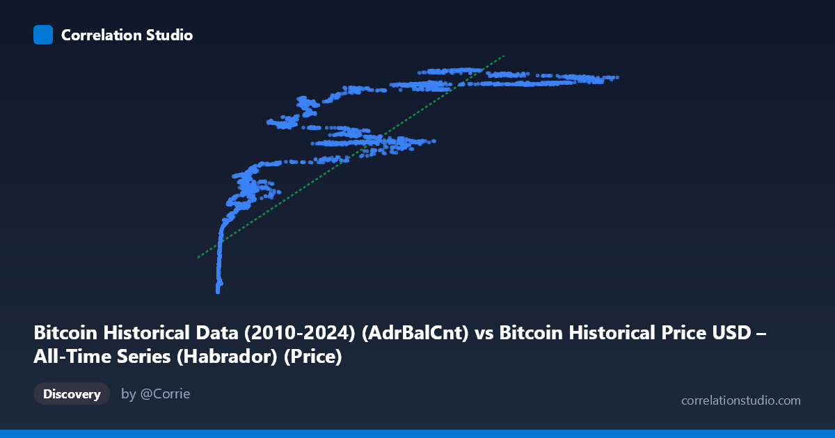
Bitcoin Historical Data (2010-2024) (AdrBalCnt) vs Bitcoin Historical Price USD – All-Time Series (Habrador) (Price)
- Pearson correlation (r)
- 0.8326
- Spearman correlation
- 0.9741
- p-value
- 0
- Sample size (n)
- 5789
- 95% confidence interval
- 0.8245 to 0.8403
- Granger causality
- None
- Granger optimal lag
- 10
- Time coverage
- 2010-07-18 to 2026-05-23
- Recomputed on refreshed data
- 2026-10-24 (r was 0.8303)
AI analysis
Analysis: Bitcoin Active Address Count vs. Price
1. Relationship Overview
The scatterplot shows a strong positive association between Bitcoin's active address count (X) and its USD price (Y), but the relationship is clearly non-linear. At low address counts (under ~1,000), prices cluster tightly near zero (tens of thousands of dollars), while at high address counts (tens of thousands), prices span a much wider range (roughly $20M–$57M in this scaled dataset). This fan-shaped dispersion — tight at low X, wide at high X — is a classic signature of heteroscedasticity and suggests a logarithmic or power-law relationship rather than a simple linear one, consistent with the note that Spearman ρ exceeds Pearson r.
2. Strength, Direction, and Statistical Confidence
The Pearson correlation (r = 0.83) is strong and positive, with r² = 0.69 indicating that address activity linearly explains about 69% of the variance in price — leaving roughly 31% driven by other factors (market sentiment, macro liquidity, halving cycles, regulatory news, etc.). The 95% CI [0.822, 0.838] is narrow, and the p-value is effectively 0, so the correlation itself is highly reliable given the large sample (n = 5,764). However, the Granger causality test found no significant predictive direction in either direction (X→Y: p = 0.95; Y→X: p = 0.73) at 10 lags. This is a critical caveat: strong contemporaneous correlation does not imply that address growth predicts price, or vice versa. Both series likely co-move because they are jointly driven by an underlying trend (network adoption/hype cycles) rather than one causing the other in a lagged, forecastable sense.
3. Notable Patterns and Outliers
Several features stand out: - Saturation at high X: Beyond ~60,000–90,000 addresses, price plateaus around $53–57M despite continued increases in address count — suggesting diminishing marginal price impact per new address, or a price ceiling within this data window. - Vertical banding: Multiple points with similar X (e.g., ~87,000–94,000 addresses) show varying Y values ($53M–$57M), indicating price is influenced by additional time-varying factors beyond raw address count on any given day. - Low-X cluster: A dense clump near X < 20 with Y under $1M likely represents Bitcoin's earliest years (2010–2011), which may be exerting disproportionate leverage on the linear fit. - Extreme range compression: X spans from 0.05 to 124,720 (a 5-order-of-magnitude range) while Y spans a comparable multi-order range — reinforcing that a log-log transformation would likely linearize the relationship and improve fit.
4. Confounders and Caveats
This is fundamentally a time-series correlation, not a cross-sectional one — both variables trend upward over 2010–2026 alongside overall market maturation, adoption, and macro liquidity cycles. This creates classic spurious correlation risk via co-trending: many unrelated growing time series would show similarly high r purely from shared upward drift, not genuine mechanistic linkage. Address count itself is a noisy proxy for "network usage" (it can be inflated by exchange consolidation, wallet-splitting behavior, or bot activity) and doesn't capture transaction value or velocity. Additionally, price is exposed to exogenous shocks (regulatory announcements, ETF approvals, macro rate changes) uncorrelated with organic address growth, which likely explains both the residual 31% unexplained variance and the lack of Granger causality.
5. Recommendations
- Refit with log or power-law transformation (e.g., log(Y) ~ log(X)) given the fan-shaped residuals and Spearman Pearson signal; this should meaningfully improve R² and better reflect the network-adoption dynamics (similar to Metcalfe's Law framings of crypto valuation). - Detrend or difference both series (e.g., % daily change) before testing causality, since Granger tests on non-stationary trending data are unreliable and can mask true short-term lead-lag relationships. - Segment by market cycle/halving era (2010–2013, 2013–2017, 2017–2021, 2021–2024) to check whether the X-Y relationship is stable or regime-dependent — the plateau near max X hints the relationship may differ by cycle. - Incorporate additional covariates (transaction count, realized cap, exchange volume) in a multivariate model to isolate address count's marginal explanatory power beyond general market trend.
X dataset: Bitcoin Historical Price USD – All-Time Series (Habrador)
Y dataset: Bitcoin Historical Data (2010-2024)
Part of experiment: Bitcoin - Bitcoin Historical Price USD – All-Time Series (Habrador) vs Bitcoin Historical Data (2010-2024)