VIX Volatility Index Daily (FRED) (VIXCLS) vs Cboe U.S. Equities Historical Market Volume Data 2010 (Tape A Notional)
- Pearson correlation (r)
- 0.4463
- Spearman correlation
- 0.2184
- p-value
- 0
- Sample size (n)
- 252
- 95% confidence interval
- 0.3415 to 0.5401
- Granger causality
- Y → X
- Granger optimal lag
- 1
AI analysis
Analysis: VIX Volatility Index vs. Cboe U.S. Equities Market Volume (2010)
Relationship Overview
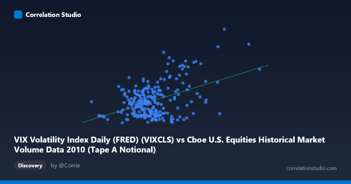
The scatterplot reveals a moderate positive relationship between daily U.S. equity market notional trading volume (X-axis) and the VIX Volatility Index (Y-axis) across 2010. As market volume increases, VIX levels tend to rise, which aligns intuitively with the well-established financial principle that heightened market uncertainty drives both fear (VIX) and trading activity simultaneously. The linear regression equation (y = 9.75×10⁻¹⁰x + 13.70) indicates that for every ~1 trillion dollars increase in notional volume, VIX rises by approximately 0.975 points, with a baseline VIX of roughly 13.7 at minimal volume levels.
Correlation Strength and Statistical Significance
The Pearson correlation of r = 0.4463 reflects a moderate positive association, but the coefficient of determination (r² = 0.1992) is the more sobering metric — only ~20% of the variance in VIX is explained by trading volume, leaving 80% attributable to other factors. The 95% confidence interval [0.3415, 0.5401] is reasonably tight and does not approach zero, and the p-value of 9.75×10⁻¹⁴ confirms the relationship is highly statistically significant with near-zero probability of occurring by chance across n=252 paired observations. Critically, the Granger causality results indicate a unidirectional temporal relationship: Y Granger-causes X (F=9.63, p=0.0021), meaning past VIX values predict future trading volume, but not the reverse (X→Y: p=0.073, non-significant at α=0.05). This is a meaningful finding — fear and implied volatility precede elevated trading activity, suggesting investors react to volatility signals by increasing their trading behavior with a one-period lag.
Patterns, Clusters, and Outliers
The scatterplot exhibits several notable structural features. The bulk of observations cluster between ~5–12 billion in notional volume and VIX levels of 15–27, representing "normal" 2010 market conditions. However, there is a clear upper-right cluster of high-leverage outliers — points with volumes exceeding ~14–19 billion and VIX readings of 35–46 — that exert considerable influence on the positive slope. These likely correspond to specific volatility episodes in 2010, most notably the May 6th "Flash Crash" and the European sovereign debt crisis flare-ups in spring and summer. There also appears to be a lower-left cluster with modest volumes (4–7 billion) yet varying VIX readings (15–26), suggesting that low-volume periods are not consistently associated with low fear. The scatter fan widens at higher volume levels, indicating possible heteroscedasticity — variance in VIX is not constant across the volume range, which mildly undermines the linear model's assumptions.
Confounding Factors and Caveats
Several important caveats should temper interpretation. First, reverse causality is plausible even beyond the Granger result — high VIX triggers algorithmic and institutional trading programs that mechanically increase volume, making the causal arrow difficult to isolate cleanly. Second, omitted variable bias is substantial: macroeconomic news releases (Fed announcements, non-farm payrolls), geopolitical events, and options expiration cycles independently drive both VIX and volume without one causing the other. Third, the dataset covers only one calendar year (2010), a period with idiosyncratic events (Flash Crash, EU debt crisis), limiting generalizability. Fourth, the VIX and notional volume data come from different source datasets with different primary purposes, introducing potential temporal alignment and aggregation mismatches. Finally, notional volume conflates price levels and share count — a rising market inflates notional figures even at constant share volume, potentially introducing a price-level artifact into the X variable.
Actionable Insights and Further Investigation
Practitioners and researchers should consider several follow-up directions. Given the Granger causality finding, VIX could be incorporated as a leading indicator in intraday or next-day trading volume forecasting models, particularly for market microstructure or liquidity planning purposes. It would be valuable to extend the analysis across multiple years (2008–2023) to test whether the r=0.45 relationship holds across different volatility regimes, especially ultra-low VIX environments (2017) versus crisis periods (2008, 2020). Segmenting the data by market regime (VIX <15, 15–25, 25) would clarify whether the relationship is being driven predominantly by tail events. Researchers should also control for day-of-week effects, options expiration dates, and macro announcement days as covariates in a multivariate regression to isolate the true volume-volatility relationship. Finally, applying a log transformation to the X variable (notional volume spans a wide range) may address heteroscedasticity and improve model fit beyond the current 20% explained variance.
X dataset: Cboe U.S. Equities Historical Market Volume Data 2010
Y dataset: VIX Volatility Index Daily (FRED)
Part of experiment: Daily - Cboe U.S. Equities Historical Market Volume Data 2010 vs VIX Volatility Index Daily (FRED)