Nikkei 225 Stock Average (NIKKEI225) vs Cboe U.S. Equities Historical Market Volume Data 2009 (Tape C Trade Count)
- Pearson correlation (r)
- -0.4381
- Spearman correlation
- -0.4325
- p-value
- 0
- Sample size (n)
- 235
- 95% confidence interval
- -0.5361 to -0.3286
- Granger causality
- None
- Granger optimal lag
- 10
AI analysis
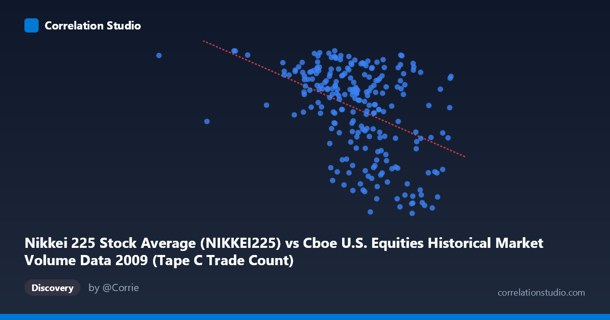
Scatterplot Analysis: Nikkei 225 vs. Cboe Tape C Trade Count (2009)
Relationship Overview
The scatterplot reveals a moderate negative relationship between the Nikkei 225 index level and the Cboe U.S. Equities Tape C trade count across 2009. As the Nikkei 225 rises, U.S. equity trade counts on Tape C tend to decline. This is a somewhat counterintuitive finding at first glance — one might expect rising Japanese equity prices to coincide with buoyant global market activity — but the pattern likely reflects the turbulent recovery dynamics of 2009, where market stabilization reduced the frantic trading volumes that characterized the crisis period. The regression line (y = −0.00431x + 12,094.9) confirms this downward slope, though the scatter around the line is substantial, indicating that the linear model captures only part of the story.
Correlation Strength, Direction, and Causality
The Pearson correlation of r = −0.438 indicates a moderate negative association, statistically significant with a p-value of 1.93 × 10⁻¹², which is extraordinarily small and effectively rules out chance as an explanation given the sample of n = 235. However, statistical significance here is partly a function of the large population (N = 3,232), so practical significance deserves equal scrutiny. The R² of 0.192 means that Nikkei 225 levels explain only about 19.2% of the variance in Tape C trade counts — meaning roughly 80.8% of the variation remains unexplained by this relationship alone. The 95% confidence interval for r of [−0.536, −0.329] is moderately wide, suggesting meaningful uncertainty in the precise strength of the association. Critically, the Granger causality tests found no significant predictive directionality in either direction (X→Y: F = 1.83, p = 0.057; Y→X: F = 1.81, p = 0.061), with both p-values tantalizingly close to but not crossing the 0.05 threshold. This means neither variable reliably predicts the other temporally — the correlation is contemporaneous and likely driven by shared external forces rather than a direct lead-lag mechanism.
Notable Patterns, Clusters, and Outliers
The sample points reveal considerable heteroscedasticity and non-linearity. There is a dense cluster of observations in the X range of roughly 580,000–720,000 (Nikkei values) paired with a wide spread of trade counts from ~7,200 to ~10,600, suggesting high variability in U.S. trading activity even when the Nikkei is at similar levels. Several notable outliers are visible: points at very low Nikkei values (e.g., ~294,700 and ~470,000–510,000) tend to pair with higher trade counts (~9,000–10,400), consistent with the early-2009 crisis environment when panic selling drove extreme volumes. Conversely, some high-Nikkei observations (e.g., ~841,895 and ~824,368) show moderate-to-high trade counts, suggesting the relationship may weaken or reverse at the upper tail. The point near (761,868, 7,280) stands out as a low-trade-count outlier at a relatively high Nikkei level.
Confounding Factors and Caveats
Several important caveats apply. First, 2009 was a structurally unique year — spanning the trough of the Global Financial Crisis in early Q1 and a dramatic recovery rally through year-end — meaning temporal trends in both series (declining volatility, rising prices) could be producing a spurious correlation driven by shared time trends rather than any direct economic linkage. Second, the axis labels appear swapped in the dataset metadata (Nikkei data is labeled as a Cboe dataset column and vice versa), warranting verification of data provenance before drawing conclusions. Third, Tape C trade counts reflect NYSE Arca-listed securities specifically, not total U.S. market volume, limiting generalizability. Fourth, currency effects, time-zone differences between Japanese and U.S. markets, and macroeconomic co-movement (risk-on/risk-off sentiment) are all potential confounders that could independently drive both variables.
Actionable Insights and Further Investigation
Given that ~80% of variance is unexplained and Granger causality is absent, this correlation should not be used as a predictive trading signal between these two markets. However, the relationship is worth deeper investigation. Researchers should consider: (1) detrending both series to remove the shared 2009 recovery trend before recalculating correlation; (2) segmenting the year into crisis (Q1), stabilization (Q2), and recovery (Q3–Q4) phases to test whether the correlation is stable or regime-dependent; (3) incorporating VIX or volatility measures as a potential common driver; and (4) expanding the analysis to multiple years to determine whether the negative relationship persists beyond this structurally anomalous period. The near-significant Granger results (p ≈ 0.057–0.061) also suggest that a slightly longer lag window or larger sample might reveal weak predictive structure worth monitoring.
X dataset: Cboe U.S. Equities Historical Market Volume Data 2009
Y dataset: Nikkei 225 Stock Average
Part of experiment: Daily - Cboe U.S. Equities Historical Market Volume Data 2009 vs Nikkei 225 Stock Average