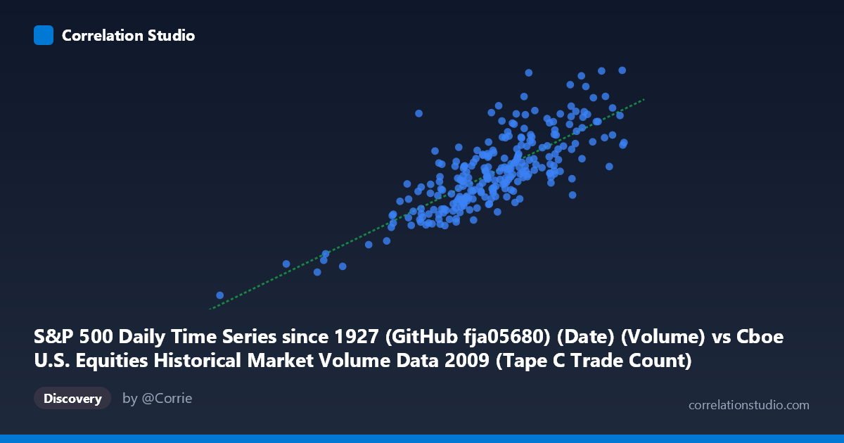
S&P 500 Daily Time Series since 1927 (GitHub fja05680) (Date) (Volume) vs Cboe U.S. Equities Historical Market Volume Data 2009 (Tape C Trade Count)
- Pearson correlation (r)
- 0.7829
- Spearman correlation
- 0.7587
- p-value
- 0
- Sample size (n)
- 252
- 95% confidence interval
- 0.73 to 0.8265
- Granger causality
- None
- Granger optimal lag
- 10
AI analysis
Scatterplot Analysis: S&P 500 Trading Volume vs. Cboe Tape C Trade Count (2009)
Relationship Overview The scatterplot reveals a clear positive linear relationship between daily S&P 500 trading volume (X-axis) and Cboe U.S. Equities Tape C trade count (Y-axis) across 252 trading days in 2009. As overall market volume increases, the number of discrete trades recorded on Tape C rises proportionally, which is broadly intuitive — higher aggregate market activity naturally generates more individual transactions. The linear regression equation (y = 10,303.7x − 978,275,000) suggests that for every additional unit of S&P 500 volume, Tape C trade count increases by approximately 10,304 trades, though the intercept's negative value implies the relationship only becomes meaningful above a certain volume threshold.
Correlation Strength and Statistical Significance The Pearson correlation of r = 0.7829 indicates a strong positive association, and the coefficient of determination r² = 0.6130 tells us that approximately 61.3% of the variance in Tape C trade count is explained by S&P 500 trading volume — a substantial but incomplete explanatory share, meaning roughly 38.7% of variation stems from other sources. The 95% confidence interval of [0.7300, 0.8265] is relatively tight and lies well above zero, reinforcing reliability. The p-value of effectively zero confirms this correlation is highly unlikely to be a chance finding across the n = 252 paired observations drawn from the N = 3,232 population. However, Granger causality tests reveal no significant temporal predictive direction in either direction (X→Y: F = 1.03, p = 0.42; Y→X: F = 0.79, p = 0.64), even at an optimal lag of 10 periods. This is a critical qualifier: while the two series move together contemporaneously, neither reliably leads the other, suggesting they respond jointly to shared market forces rather than one driving the other.
Notable Patterns, Clusters, and Outliers The data points form a reasonably coherent linear band, but with noticeable vertical dispersion, particularly in the mid-to-upper volume range (600,000–750,000), where Tape C trade counts span a wide range (roughly 4.0B to 8.6B). This heteroscedasticity — increasing spread at higher X values — suggests the relationship becomes less predictable at elevated volume levels. Two points stand out as potential outliers: the upper-right cluster anchored near (845,583; 9.12B) and (778,644; 8.93B) represents extreme high-activity days, likely corresponding to late 2008/early 2009 volatility spillovers or major macroeconomic announcements. Conversely, the lower-left point at approximately (185,887; 1.27B) is a dramatic outlier — far removed from the main cluster — and likely represents a holiday-shortened session or data anomaly. A modest concentration of points exists in the 580,000–700,000 volume range, reflecting typical 2009 trading conditions post-crisis stabilization.
Confounding Factors and Caveats Several important caveats temper interpretation. First, Tape C specifically covers NYSE Arca-listed securities, meaning it captures only a subset of total market activity; the strong correlation may partly reflect structural co-movement across all venues rather than a direct causal mechanism. Second, 2009 was an exceptional year — spanning the tail of the financial crisis and a historic market recovery — so elevated and volatile volume figures may produce correlations that do not generalize to normal market regimes. Third, the negative Granger causality result at up to 10 lags suggests both series are likely driven by a common latent factor (e.g., macroeconomic news, VIX-driven risk sentiment, or Federal Reserve announcements) rather than exhibiting independent predictive power. Finally, the dataset conflates volume (shares traded) with trade count (number of transactions), and changes in average trade size — driven by algorithmic fragmentation trends — could artificially inflate or deflate the relationship over time.
Actionable Insights and Further Investigation Practitioners and researchers should avoid assuming directional predictability from this correlation for trading or risk models, given the Granger causality null result. Instead, the relationship is more useful as a contemporaneous monitoring signal — unusually divergent readings between aggregate volume and Tape C trade count on a given day may flag fragmentation anomalies or venue-specific disruptions worth investigating. Further analysis should: (1) control for VIX or realized volatility as a potential common driver; (2) extend the time window beyond 2009 to test whether the r = 0.78 correlation holds in lower-volatility regimes; (3) examine residuals from the linear model to identify whether specific event dates (FOMC meetings, earnings seasons) systematically explain the unexplained 38.7% variance; and (4) test non-linear models (e.g., log-log or polynomial regression) given the apparent heteroscedasticity, which may improve both fit and interpretability across the full volume range.
X dataset: Cboe U.S. Equities Historical Market Volume Data 2009
Y dataset: S&P 500 Daily Time Series since 1927 (GitHub fja05680) (Date)
Part of experiment: Daily - Cboe U.S. Equities Historical Market Volume Data 2009 vs S&P 500 Daily Time Series since 1927 (GitHub fja05680) (Date)