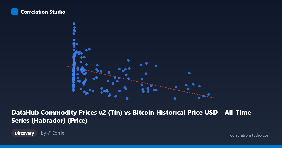
DataHub Commodity Prices v2 (Tin) vs Bitcoin Historical Price USD – All-Time Series (Habrador) (Price)
- Pearson correlation (r)
- -0.425
- Spearman correlation
- -0.31
- p-value
- 0
- Sample size (n)
- 182
- 95% confidence interval
- -0.5373 to -0.298
- Granger causality
- None
- Granger optimal lag
- 1
AI analysis
Analysis: Bitcoin Price vs. Tin Commodity Price
1. Relationship Overview
The scatterplot shows a modest negative relationship between Bitcoin price (X-axis) and tin commodity price (Y-axis) across 182 paired monthly observations from 2010–2025. At low Bitcoin prices (below ~$1,000), tin prices span the full range of the dataset (6.6–10.75), including several high outliers above 9.0–10.75. As Bitcoin prices climb into the tens of thousands, tin prices compress into a narrower, lower band (roughly 6.6–8.7), with most points clustering between 6.8–8.0. This creates a fan-shaped or converging pattern rather than a clean linear trend.
2. Strength, Direction, and Statistical Confidence
The correlation coefficient (r = -0.425) indicates a weak-to-moderate negative relationship. The r² of 0.181 means only about 18% of the variance in tin prices is statistically explained by Bitcoin price levels — leaving over 80% of tin's price variation attributable to other factors. The 95% CI [-0.537, -0.298] is reasonably tight and entirely negative, and the p-value (2.22E-09) confirms this correlation is highly unlikely due to chance. However, statistical significance here reflects the large historical span and monotonic trends in both series (Bitcoin's long-term rise, tin's relative stability) rather than a strong functional relationship. Critically, Granger causality tests show no significant predictive direction in either direction (X→Y: p=0.29; Y→X: p=0.18). This is important: despite the correlation, neither series meaningfully helps forecast the other's future values — the relationship is likely coincidental co-trending rather than causal or lead-lag dynamic.
3. Patterns and Outliers
Several notable features stand out: - Early-period volatility cluster: Many high-Y outliers (Y 9.0, including 10.75, 10.40, 10.36, 10.32) occur when Bitcoin was under $1,000 — likely reflecting a specific tin price spike or index rebasing early in the sample period, independent of Bitcoin dynamics. - Compression at high X: Once Bitcoin exceeds ~$20,000, tin values narrow considerably (mostly 6.6–8.7), suggesting reduced variance rather than a strict linear decline. - No clear non-linear curve: The pattern doesn't suggest a strong power-law or logarithmic fit; it looks more like two different variance regimes (high-variance early period, low-variance later period) coinciding with Bitcoin's price scale.
4. Confounding Factors and Caveats
This correlation is almost certainly spurious or indirect, driven by shared time-trends rather than genuine economic linkage: - Common time trend confound: Bitcoin has trended upward over 15 years while tin has been comparatively range-bound; any two time series with differing long-term trends can show artificial correlation. - Macroeconomic co-drivers: Global liquidity conditions, USD strength, inflation expectations, and interest rates could simultaneously influence both crypto speculation and industrial metal pricing without one causing the other. - Non-stationarity: Neither series is likely stationary (Bitcoin especially), which can inflate correlation and bias Granger causality tests unless differenced. The tests presented should be interpreted cautiously. - Monthly aggregation and mismatched scales: Bitcoin's extreme right-skewed distribution (mean $17,943, stdev $27,080) versus tin's compact range invites regression distortion; log-transforming Bitcoin would likely be more appropriate.
5. Suggested Next Steps
Given the lack of Granger causality and weak r², this correlation should not be used for trading or forecasting purposes. To clarify whether any genuine relationship exists: - Log-transform Bitcoin prices before correlation/regression analysis, given its exponential growth pattern. - Difference or detrend both series (e.g., use % monthly returns instead of price levels) and re-run correlation and Granger tests to remove spurious trend-driven correlation. - Test against a common macro factor (e.g., DXY dollar index, real interest rates, global M2 money supply) to see if it explains both series better than they explain each other. - Segment analysis by era (2010–2017 vs. 2018–2025) to check if the relationship is era-specific or an artifact of early low-liquidity tin pricing data.
X dataset: Bitcoin Historical Price USD – All-Time Series (Habrador)
Y dataset: DataHub Commodity Prices v2
Part of experiment: Bitcoin - Bitcoin Historical Price USD – All-Time Series (Habrador) vs DataHub Commodity Prices v2