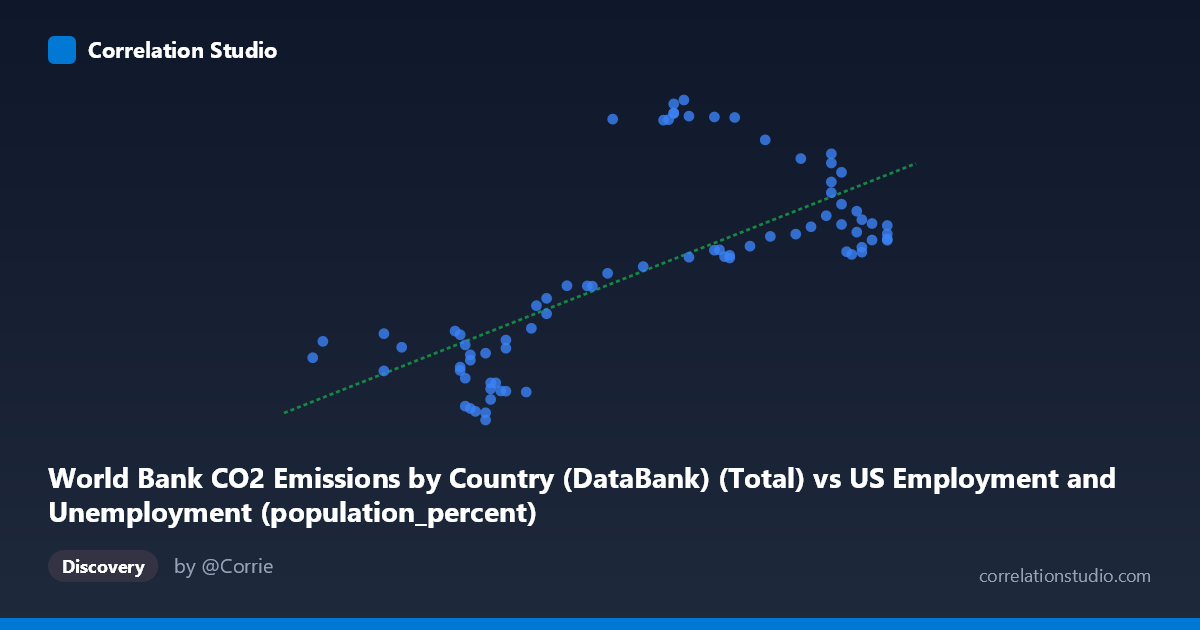
World Bank CO2 Emissions by Country (DataBank) (Total) vs US Employment and Unemployment (population_percent)
- Pearson correlation (r)
- 0.7123
- Spearman correlation
- 0.7223
- p-value
- 0
- Sample size (n)
- 80
- 95% confidence interval
- 0.584 to 0.8059
- Granger causality
- Y → X
- Granger optimal lag
- 10
- Time coverage
- 1941-01-01 to 2020-01-01
AI analysis
Scatterplot Analysis: US Employment Rate vs. CO₂ Emissions
1. Overall Relationship
The scatterplot reveals a moderate-to-strong positive relationship between US employment/unemployment population percentage (X-axis) and CO₂ fossil fuel emissions (Y-axis), spanning data from 1941 to 2020. As the employment-related metric increases from roughly 55.8 to 67.1, CO₂ emissions trend upward from approximately 9,870 to 43,129 units. The fitted linear regression (y = 2087.02x − 104,678) captures a general upward trajectory, though the scatter around this line is substantial and clearly non-uniform, suggesting the relationship is more complex than a simple linear association.
2. Correlation Strength, Direction, and Causality
The Pearson correlation of r = 0.712 indicates a moderately strong positive association, but the coefficient of determination r² = 0.507 is the more sobering statistic — only ~51% of the variance in CO₂ emissions is explained by the employment metric, meaning roughly half the variation in emissions is driven by factors entirely outside this model. The 95% confidence interval for r of [0.584, 0.806] confirms the association is reliably positive but spans a meaningful range, reflecting genuine uncertainty. The p-value of 1.27×10⁻¹³ makes it statistically unambiguous that this correlation did not arise by chance given n = 80 paired observations. Critically, the Granger causality analysis points unidirectionally: Y Granger-causes X (F = 2.31, p = 0.026) with an optimal lag of 10 periods, while X→Y is non-significant (F = 1.17, p = 0.331). This is a striking and counterintuitive result — it suggests that past CO₂ emission levels carry predictive information about future employment rates, not the reverse. This temporal directionality warrants serious scrutiny before any causal narrative is constructed.
3. Notable Patterns, Clusters, and Outliers
The scatterplot reveals at least two distinct behavioral clusters rather than a clean continuum: - A lower-left cluster (X ≈ 56–61, Y ≈ 10,000–22,000) where points are relatively tightly grouped with modest emissions - An upper zone (X ≈ 61–67, Y ≈ 25,000–43,000) where emissions spread widely — notably, several points at similar X values (e.g., X ≈ 62.8–63.2) show Y values ranging from ~26,000 to ~43,000, implying high vertical dispersion at mid-to-high X values
Several high-leverage outliers are apparent, particularly the cluster of points near (62.7–63.2, 41,000–43,129) that sit well above the regression line, and conversely, points like (67.1, 28,551) and (66.5, 29,394) that fall considerably below it. This fan-shaped or heteroscedastic spread — variance in Y increasing with X — suggests a potential non-linear or multiplicative underlying process that a simple linear fit inadequately captures.
4. Confounding Factors and Interpretive Caveats
Several important caveats apply. First, this correlation likely reflects shared secular trends: both employment rates and CO₂ emissions co-evolved with post-WWII US economic expansion, industrialization, and population growth over 80 years — a classic spurious correlation driven by a common temporal confounder. Second, the dataset description contains an apparent variable labeling inconsistency: the X-axis is labeled as CO₂ emissions yet sourced from a US employment dataset, and the Y-axis as employment percentage yet sourced from a CO₂ dataset — this warrants verification of whether the axes reflect the intended variables. Third, the Granger causality result (Y→X) may itself be an artifact of shared macroeconomic cycles rather than a genuine mechanism; Granger causality tests temporal precedence, not true causation. Finally, aggregating global CO₂ data with US-specific employment figures introduces a geographic mismatch that could mask or inflate apparent relationships.
5. Actionable Insights and Further Investigation
Given these findings, several next steps are warranted: - Detrend both time series (e.g., first-differencing or HP filter) to remove shared secular trends and test whether the correlation persists independently of long-run drift - Investigate the outlier cluster around X ≈ 62.7–63.2 to determine whether these correspond to specific historical periods (e.g., economic booms, energy crises, COVID-era disruptions) - Test non-linear models (polynomial, log-log, or piecewise regression) given the apparent heteroscedasticity and clustering - Introduce control variables such as GDP, energy prices, industrial output, and population to partial out confounding economic drivers - Verify the Granger lag structure across multiple lag specifications and apply cointegration testing (e.g., Johansen or Engle-Granger) to determine whether a long-run equilibrium relationship exists — which would have meaningful implications for emissions forecasting using labor market indicators
X dataset: US Employment and Unemployment
Y dataset: World Bank CO2 Emissions by Country (DataBank)
Part of experiment: Yearly - US Employment and Unemployment vs World Bank CO2 Emissions by Country (DataBank)