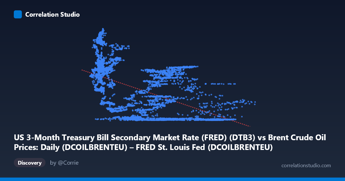
US 3-Month Treasury Bill Secondary Market Rate (FRED) (DTB3) vs Brent Crude Oil Prices: Daily (DCOILBRENTEU) – FRED St. Louis Fed (DCOILBRENTEU)
- Pearson correlation (r)
- -0.5411
- Spearman correlation
- -0.5787
- p-value
- 0
- Sample size (n)
- 9642
- 95% confidence interval
- -0.555 to -0.5268
- Granger causality
- None
- Granger optimal lag
- 1
AI analysis
Analysis: US 3-Month T-Bill Rate vs. Brent Crude Oil Price (1987–2026)
Relationship Overview
The scatterplot reveals a moderate negative relationship between the US 3-Month Treasury Bill rate (X-axis) and Brent Crude Oil prices (Y-axis), summarized by the linear regression equation y = -0.041x + 5.10. As T-bill rates rise, crude oil prices tend to fall — and vice versa. However, the data cloud is notably wide and heteroscedastic, with substantial scatter across nearly all X values. The X range spans roughly 9 to 144 (likely basis points or percentage × 10), while Y (oil prices, USD/barrel) ranges from near zero to ~$9 in the normalized or transformed scale shown. The relationship is real but far from deterministic, and the raw scatter immediately signals that many other forces are simultaneously driving oil prices.
Correlation Strength, Direction, and Causality
The Pearson correlation of r = −0.54 indicates a moderate negative association, but the variance-explained metric tells a more sobering story: R² = 0.293, meaning T-bill rates account for only about 29% of the variance in Brent crude prices, leaving 71% unexplained by this single predictor. The 95% confidence interval of [−0.555, −0.527] is narrow given the large paired sample (n = 9,642), and the p-value of effectively zero confirms the correlation is highly statistically significant — not a sampling artifact. That said, statistical significance here is largely a function of enormous sample size and should not be conflated with practical or economic significance. Critically, the Granger causality tests find no significant predictive direction in either direction (X→Y: F = 1.73, p = 0.189; Y→X: F = 0.005, p = 0.944), meaning neither series reliably predicts the other at the optimal 1-period lag. This is an important caveat: the cross-sectional correlation exists, but it carries no demonstrated temporal forecasting power.
Notable Patterns, Clusters, and Non-Linearity
Several structural features stand out in the sample points. There is a pronounced cluster of low-X, high-Y observations (e.g., X ≈ 14–22, Y ≈ 5–9), consistent with the post-2008 and post-2020 era of near-zero interest rates coinciding with volatile but sometimes elevated oil prices. Conversely, high-X values (X 60–100) almost universally pair with very low Y values (near zero to ~5), suggesting that high-rate regimes historically corresponded to lower oil price levels — plausibly the 1990s era of lower crude prices. Several outliers are visible: points like (19.90, 8.81), (19.75, 8.82), and (86.82, 5.33) deviate notably from the regression line, hinting at oil price spikes (likely Gulf War 1990, COVID recovery 2021–2022, or Russia-Ukraine 2022) that occurred regardless of the rate environment. The relationship also appears non-linear — the decline in Y as X increases is steep at low X values but flattens at higher X, suggesting a potential log or inverse functional form would outperform the linear model.
Confounding Factors and Interpretive Caveats
The negative correlation almost certainly reflects shared macroeconomic regime effects rather than a direct causal mechanism. Both variables are jointly driven by the broader business cycle: recessions tend to suppress oil demand (lowering prices) while also prompting Fed rate cuts (lowering T-bill rates) — which would actually produce a positive co-movement. The observed negative correlation may instead reflect that high-rate periods (1990s) historically coincided with structurally lower oil prices, while the low-rate post-2008 era saw oil prices elevated by emerging market demand, geopolitical supply disruptions, and OPEC policy. The axis labeling appears swapped from the dataset descriptions (X is labeled as T-bill rate but the dataset title says "Brent Crude" and vice versa) — this warrants verification before drawing conclusions. Additionally, both series span nearly four decades with profound structural breaks (Gulf War, 9/11, 2008 GFC, COVID-19, Ukraine war), meaning the correlation may be non-stationary and vary substantially across sub-periods.
Actionable Insights and Further Investigation
Given these findings, several investigative steps would add significant analytical value. First, segment the analysis by economic regime or decade to test whether the correlation is stable or driven by a specific historical period — a rolling-window correlation would reveal this clearly. Second, test non-linear specifications (logarithmic, inverse, or piecewise regression) given the apparent curvature in the scatterplot; the linear R² of 29.3% may improve meaningfully. Third, introduce control variables such as USD index, global GDP growth, OPEC production levels, and inflation expectations to partial out confounding macro factors and isolate any residual T-bill/crude relationship. Fourth, extend Granger causality testing to longer lags (e.g., 3–12 months) since monetary policy transmits to commodity markets with well-documented delays. Finally, consider cointegration analysis to test whether these series share a long-run equilibrium relationship despite the lack of short-term Granger causality — a more appropriate tool for two non-stationary financial time series spanning 38 years.
X dataset: Brent Crude Oil Prices: Daily (DCOILBRENTEU) – FRED St. Louis Fed
Y dataset: US 3-Month Treasury Bill Secondary Market Rate (FRED)
Part of experiment: Daily - Brent Crude Oil Prices: Daily (DCOILBRENTEU) – FRED St. Louis Fed vs US 3-Month Treasury Bill Secondary Market Rate (FRED)