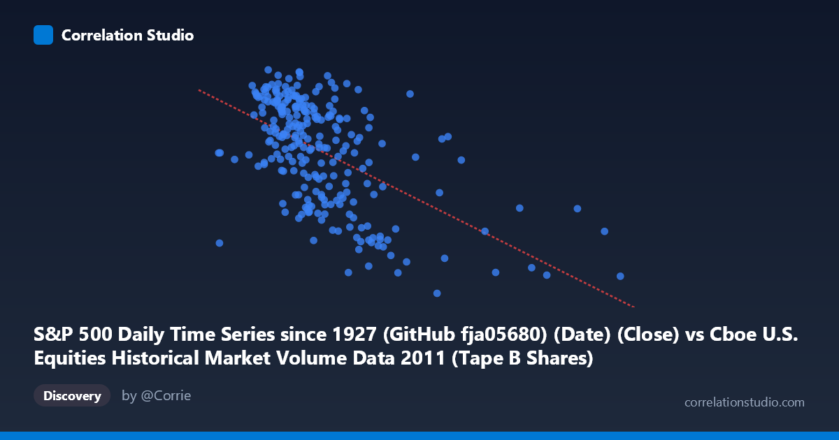
S&P 500 Daily Time Series since 1927 (GitHub fja05680) (Date) (Close) vs Cboe U.S. Equities Historical Market Volume Data 2011 (Tape B Shares)

Pearson correlation (r): -0.5574
Spearman correlation: -0.5372
p-value: 0
Sample size (n): 252
95% confidence interval: -0.6371 to -0.466
Granger causality: None
Granger optimal lag: 1

AI analysis

Scatterplot Analysis: S&P 500 Close Price vs. Cboe Tape B Share Volume (2011)

Relationship Overview The scatterplot reveals a negative relationship between the S&P 500 daily closing price (X-axis) and Cboe Tape B share volume (Y-axis) across 252 trading days in 2011. As the S&P 500 index level rises, Tape B share volume tends to decrease, and conversely, lower index values are associated with higher trading volumes. This inverse pattern is consistent with a well-documented market phenomenon: elevated trading activity often coincides with periods of market stress, uncertainty, or drawdown, rather than during calm, rising markets. The linear regression equation (y = -1.059×10⁻⁶x + 1371.6) confirms this downward slope, suggesting that for every 10-million-point increase in the index closing value, Tape B shares decline by approximately 10.6 units on average.

Correlation Strength, Direction, and Statistical Context The Pearson correlation coefficient of r = -0.5574 indicates a moderate negative correlation. While directionally meaningful, the coefficient of determination r² = 0.3107 tells a more tempered story: S&P 500 closing prices explain only 31.1% of the variance in Tape B share volume, leaving nearly 69% attributable to other factors. The 95% confidence interval of [-0.6371, -0.4660] is meaningfully narrow and entirely negative, confirming that the direction of the relationship is reliable and not a statistical artifact. With a p-value effectively at 0 and a sample of n = 252 drawn from a population of N = 3,780, the correlation is highly statistically significant. However, the Granger causality results tell a critical story: neither direction (X→Y: F = 0.133, p = 0.716; Y→X: F = 0.015, p = 0.901) achieves significance, meaning that past S&P 500 prices do not reliably predict future Tape B volume, and vice versa. The relationship is contemporaneous and associative, not predictive in a temporal sense.

Notable Patterns, Clusters, and Outliers Several features stand out in the data. There is a visible cluster of high-volume observations (Tape B shares above ~1,300) concentrated at lower S&P 500 levels (roughly 60M–95M range on the X-axis), consistent with the market volatility experienced during mid-2011, when U.S. debt ceiling concerns and European sovereign debt fears drove both index declines and heightened trading. Conversely, data points with S&P 500 values exceeding ~150M show generally lower Tape B volumes. A few notable outliers are visible — particularly points near (101,941,452; 1,356.62) and (104,089,161; 1,348.65), which show high volume despite mid-range index levels, and points like (124,866,508; 1,131.42) and (120,477,249; 1,160.40), which suggest elevated index values coupled with unusually low Tape B volume. The scatter is moderately wide throughout, reinforcing that the linear model captures only a portion of the underlying dynamics.

Confounding Factors and Caveats Several important caveats apply. Tape B specifically covers NYSE American (AMEX) and regional exchange-listed securities, which may respond differently to macro conditions than the broader S&P 500 constituents. The 2011 period was unusually volatile — August 2011 saw an S&P downgrade of U.S. debt, injecting a structural regime shift that makes the year non-representative of typical market behavior. The axis labels in the dataset metadata appear potentially swapped (X is labeled as a date column "Close" from the S&P dataset, yet the X range of 41M–265M resembles volume figures), warranting careful verification of variable assignment before drawing firm conclusions. Additionally, seasonality, algorithmic trading patterns, and ETF rebalancing activity all influence Tape B volume independently of index levels, representing significant unmeasured confounders.

Actionable Insights and Further Investigation Given the moderate but incomplete correlation, several follow-up analyses are warranted. First, segmenting the data by market regime (e.g., pre- and post-August 2011 downgrade) would test whether the negative correlation is driven primarily by the stress period. Second, incorporating the VIX (volatility index) as a covariate could explain much of the residual 69% variance, as fear-driven volume spikes are likely VIX-mediated rather than price-mediated. Third, since Granger causality found no temporal predictive relationship at lag 1, testing longer lags (2–5 days) or applying a Vector Autoregression (VAR) model across multiple market indicators may uncover more nuanced dynamics. Finally, replicating this analysis across multiple years would determine whether this inverse relationship is a stable structural feature of U.S. equity markets or an artifact of 2011's exceptional conditions.

X dataset: Cboe U.S. Equities Historical Market Volume Data 2011

Y dataset: S&P 500 Daily Time Series since 1927 (GitHub fja05680) (Date)

Part of experiment: Daily - Cboe U.S. Equities Historical Market Volume Data 2011 vs S&P 500 Daily Time Series since 1927 (GitHub fja05680) (Date)