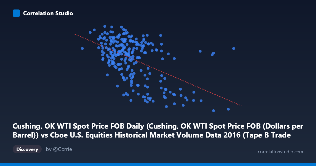
Cushing, OK WTI Spot Price FOB Daily (Cushing, OK WTI Spot Price FOB (Dollars per Barrel)) vs Cboe U.S. Equities Historical Market Volume Data 2016 (Tape B Trade Count)
- Pearson correlation (r)
- -0.5133
- Spearman correlation
- -0.4287
- p-value
- 0
- Sample size (n)
- 252
- 95% confidence interval
- -0.5988 to -0.4161
- Granger causality
- None
- Granger optimal lag
- 1
AI analysis
Analysis: WTI Crude Oil Spot Price vs. Cboe Tape B Trade Count (2016)
Relationship Overview
The scatterplot reveals a moderate negative relationship between WTI crude oil spot prices (X-axis, in dollars per barrel) and Cboe Tape B trade counts (Y-axis) across 252 trading days in 2016. As oil prices increase, trade counts on Tape B (covering NYSE American, NYSE Arca, and regional exchanges) tend to decline. The linear regression equation (y = -3.65×10⁻⁵x + 54.94) confirms this inverse slope, suggesting that for every $10 increase in WTI prices, Tape B trade counts decrease by roughly 0.365 units — though the practical magnitude depends heavily on the scale of trade count units. The relationship is visually apparent but far from deterministic, with considerable scatter throughout the plot.
Correlation Strength and Statistical Significance
The Pearson correlation of r = -0.513 indicates a moderate negative association, but the more telling statistic is r² = 0.263 — meaning WTI spot prices explain only about 26.3% of the variance in Tape B trade counts. Nearly three-quarters of the variation in trading activity is driven by factors unrelated to oil prices. The 95% confidence interval of [-0.599, -0.416] is relatively tight and excludes zero entirely, and with a p-value effectively at 0 across a population of N = 3,622, this correlation is statistically robust rather than a sampling artifact. Critically, however, Granger causality tests fail in both directions (X→Y: F = 0.608, p = 0.436; Y→X: F = 0.977, p = 0.324), meaning neither variable reliably predicts the other temporally with a one-period lag. This is a crucial caveat: the correlation reflects a contemporaneous association, not a predictive or causal mechanism.
Notable Patterns, Clusters, and Outliers
Several structural features are visible in the data. There is a dense central cluster of observations concentrated between approximately $250,000–$350,000 on the X-axis and 40–50 on the Y-axis, suggesting that most trading days in 2016 fell within a relatively stable range of both oil prices and trade volumes. However, there is a distinct lower-right tail of points — high oil price values (above ~$400,000–$550,000) paired with notably low trade counts (28–34 range) — which disproportionately drive the negative slope. Points such as (558,190, 29.55) and (467,365, 32.32) appear as potential outliers or represent a structurally different market regime. Conversely, some moderate oil price observations pair with unusually high trade counts (e.g., ~202,782, 51.44), suggesting a non-linear or threshold effect where the relationship may steepen significantly only at extreme oil price levels.
Confounding Factors and Interpretive Caveats
Several confounders complicate interpretation. 2016 was an atypical year for oil markets, spanning the tail of a major price collapse (WTI bottomed near $26/barrel in February 2016) and a partial recovery — meaning the X-axis likely captures a mean-reverting, non-stationary price series rather than random variation, which can artificially inflate or distort correlations. Tape B volume itself is influenced by algorithmic trading activity, exchange fee structures, regulatory changes, and broad market volatility (VIX), none of which are controlled for here. The note that X and Y axis dataset labels appear transposed in the metadata (the WTI price column is listed under the Cboe dataset and vice versa) warrants verification before drawing firm conclusions. Additionally, the ecological fallacy applies — a daily aggregate correlation may mask intraday or weekly patterns that behave quite differently.
Actionable Insights and Further Investigation
Despite the absence of Granger causality, the contemporaneous correlation is strong enough to warrant further investigation. Analysts should test for non-linearity (e.g., quadratic or spline regression) to determine whether the relationship is driven by extreme oil price regimes rather than being uniform across the full range. Controlling for market-wide volatility (VIX) and overall equity market volume (Tape A and C) would help isolate whether the Tape B–oil relationship is specific or simply reflects broader risk-off trading dynamics. It would also be valuable to extend the time series beyond 2016 to test whether this correlation holds across different oil price cycles. Finally, given the failed Granger causality at lag 1, testing longer lags (5–22 trading days) may reveal delayed transmission mechanisms — for instance, if sustained oil price moves take weeks to shift equity trading behavior in energy-heavy exchanges.
X dataset: Cboe U.S. Equities Historical Market Volume Data 2016
Y dataset: Cushing, OK WTI Spot Price FOB Daily
Part of experiment: Daily - Cboe U.S. Equities Historical Market Volume Data 2016 vs Cushing, OK WTI Spot Price FOB Daily