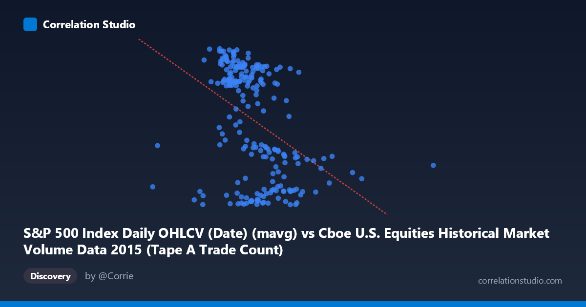
S&P 500 Index Daily OHLCV (Date) (mavg) vs Cboe U.S. Equities Historical Market Volume Data 2015 (Tape A Trade Count)
- Pearson correlation (r)
- -0.4101
- Spearman correlation
- -0.4845
- p-value
- 0
- Sample size (n)
- 222
- 95% confidence interval
- -0.514 to -0.2943
- Granger causality
- None
- Granger optimal lag
- 1
AI analysis
Analysis of S&P 500 Moving Average vs. Cboe Tape A Trade Count (2015)
Relationship Overview The scatterplot reveals a moderate negative relationship between the S&P 500 Index daily moving average (X) and the Cboe U.S. Equities Tape A Trade Count (Y) across the 2015 trading year. As the S&P 500 moving average increases, Tape A trade counts tend to decline — a counterintuitive finding at first glance, suggesting that higher index valuations in 2015 were associated with lower trading activity on Tape A venues. The linear regression equation (y = −1.006×10⁻⁵x + 135.617) quantifies this inverse slope, though the relationship is clearly not tight, with substantial scatter around the regression line throughout the range.
Correlation Strength and Statistical Significance The Pearson correlation of r = −0.41 indicates a moderate negative association, but the explanatory power is limited: r² = 0.168, meaning only ~16.8% of the variance in Tape A trade counts is explained by the S&P 500 moving average. The remaining ~83% of variability is attributable to other factors entirely. The 95% confidence interval of [−0.514, −0.294] is entirely negative and does not cross zero, and the p-value of 2.06×10⁻¹⁰ confirms the correlation is highly statistically significant — this is almost certainly not a chance finding given n = 222 paired observations. However, statistical significance should not be conflated with practical or causal significance given the modest r². Critically, Granger causality tests show no significant predictive directionality in either direction (X→Y: F = 0.49, p = 0.49; Y→X: F = 0.003, p = 0.96), meaning neither variable meaningfully predicts future values of the other at the optimal 1-period lag. This strongly cautions against any causal or predictive interpretation of the correlation.
Notable Patterns, Clusters, and Outliers Several structural features stand out in the data. The bulk of observations cluster between X values of approximately 1,100,000–1,750,000, forming a dense core with Y values spanning the full 111–130 range, which itself hints at high within-cluster variability. There are a small number of notable outliers on the far right of the X-axis — most visibly the point near (2,923,236, 115.96) and another near (2,247,816, 115.10) — which represent unusually high S&P 500 moving average values relative to the main cluster and fall on the lower end of trade counts, pulling the regression line's negative slope. These high-X outliers, if removed, could meaningfully weaken the observed correlation. There also appears to be a low-X outlier near (616,505, 118.31), isolated far to the left of the main cluster. A possible non-linear or threshold pattern may exist, where trade counts are relatively stable across a wide mid-range of index values but decline at the extremes, though the linear model does not capture this.
Confounding Factors and Interpretive Caveats Several important caveats apply. First, the X and Y axis labels appear to be swapped relative to the dataset descriptions — the moving average column is listed under the Cboe dataset while Tape A trade count is listed under the S&P 500 dataset, suggesting a potential data-joining or labeling inconsistency that warrants verification. Second, the 2015 time period was characterized by distinct market regimes — a relatively calm first half followed by the August 2015 volatility spike and year-end weakness — which could create spurious correlations driven by time-coincident trends (e.g., falling index values and changing trade volumes in August–September) rather than a true structural relationship. Third, Tape A trade counts are influenced by exchange competition, regulatory changes, and routing decisions largely independent of index level. Finally, the moving average smoothing applied to X introduces autocorrelation and lag artifacts that can distort correlation estimates.
Actionable Insights and Further Investigation Given the modest explanatory power and absent Granger causality, this correlation should not be used as a predictive signal. However, the finding is worth investigating further in several directions: (1) Segment the data by market regime (pre/post August 2015 volatility event) to test whether the correlation is driven by a specific sub-period; (2) Test for non-linear relationships (e.g., polynomial or spline regression) given the potential threshold behavior visible in the scatter; (3) Investigate and correct the dataset label mismatch to ensure the axis variables are correctly assigned; (4) Include volatility measures (e.g., VIX) as a potential mediating or confounding variable, since volatility drives both index movements and trade volumes; and (5) Examine other Tape designations (B, C) to determine whether the negative relationship is specific to Tape A or a broader market-structure phenomenon. The Granger non-result also suggests exploring longer lag structures or non-linear time-series models before concluding there is no temporal relationship.
X dataset: Cboe U.S. Equities Historical Market Volume Data 2015
Y dataset: S&P 500 Index Daily OHLCV (Date)
Part of experiment: Daily - Cboe U.S. Equities Historical Market Volume Data 2015 vs S&P 500 Index Daily OHLCV (Date)