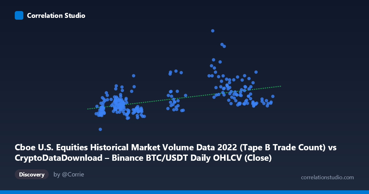
Cboe U.S. Equities Historical Market Volume Data 2022 (Tape B Trade Count) vs CryptoDataDownload – Binance BTC/USDT Daily OHLCV (Close)

Pearson correlation (r): 0.5022
Spearman correlation: 0.4963
p-value: 0
Sample size (n): 251
95% confidence interval: 0.4035 to 0.5894
Granger causality: None
Granger optimal lag: 10
Time coverage: 2022-01-03 to 2022-12-30

AI analysis

Analysis: Cboe Equities Trade Count vs. BTC/USDT Close Price

1. Overview of the Relationship

The scatterplot shows a positive but noisy relationship between the two variables—as Tape B trade counts on Cboe U.S. equities increase, BTC/USDT closing prices tend to rise as well, but the scatter around the trend line is substantial. Most points cluster in the X range of 15,000–25,000 and 40,000–45,000, with a visible gap in mid-range values (roughly 24,000–29,000), suggesting the X variable may cluster into two regimes rather than varying continuously.

2. Strength, Direction, and Uncertainty

The correlation coefficient (r = 0.502) indicates a moderate positive linear relationship, but r² = 0.252 tells the more important story: only about 25% of the variance in Y (BTC price) is explained by X (equity trade counts). The remaining 75% is driven by other factors entirely. The 95% CI [0.404, 0.589] is reasonably tight given n = 251, and the p-value of ~0 confirms the correlation is statistically significant and not due to chance—but statistical significance here should not be confused with practical predictive power, given the modest r².

Critically, the Granger causality tests show no significant predictive direction in either direction (X→Y: p = 0.382; Y→X: p = 0.505) at the optimal lag of 10 periods. This means that despite the contemporaneous correlation, neither series reliably helps forecast future values of the other. This is a common pattern with two time series that are both trending (e.g., both rising over 2022 or both influenced by a shared macro environment) without any genuine lead-lag mechanism connecting them.

3. Notable Patterns and Outliers

Several points stand out as outliers driving much of the correlation: (38730.91, 1,212,395), (36445.31, 968,367), (36958.32, 940,444), and (29103.94/29029.75, ~888,000/864,000) — these high-Y values sit well above the general cloud and appear concentrated in the X≈29,000–39,000 range. Without these points, the relationship would likely weaken further. The bulk of the data (X < 25,000 or X 40,000) shows Y values mostly confined to 350,000–680,000, with much flatter, noisier behavior. This suggests the correlation may be driven disproportionately by a handful of extreme-Y days rather than a consistent linear trend across the full range.

4. Confounding Factors and Caveats

This is a classic case of spurious correlation risk between unrelated time series. Both variables are aggregated 2022 daily data—equities trade counts and BTC prices—that could simply share common macro drivers (Fed rate decisions, risk-on/risk-off sentiment, inflation news, or simply both trending downward/upward over the year) without any direct causal link. The lack of Granger causality reinforces that this is likely correlation without causation or genuine interaction. Additionally, daily financial time series are often non-stationary (trending, autocorrelated), which can inflate correlation coefficients artificially—a well-documented pitfall when correlating two trending series without first differencing or detrending.

5. Suggested Next Steps

1. Detrend or difference both series (e.g., use daily returns/% changes instead of levels) and recompute correlation—this is essential given likely non-stationarity and will reveal if the relationship survives. 2. Investigate the high-Y outlier cluster (X ≈ 29,000–39,000) to identify specific dates—these may correspond to known BTC volatility events (e.g., FTX collapse in Nov 2022) unrelated to equity trade volume. 3. Control for shared macro variables (VIX, interest rates, overall market volume) using multivariate regression to test if the X-Y relationship holds after controlling for confounders. 4. Given the null Granger causality result, do not use this relationship for forecasting; treat any observed correlation as descriptive/contemporaneous only, not predictive.

X dataset: CryptoDataDownload – Binance BTC/USDT Daily OHLCV

Y dataset: Cboe U.S. Equities Historical Market Volume Data 2022

Part of experiment: Bitcoin - CryptoDataDownload – Binance BTC/USDT Daily OHLCV vs Cboe U.S. Equities Historical Market Volume Data 2022