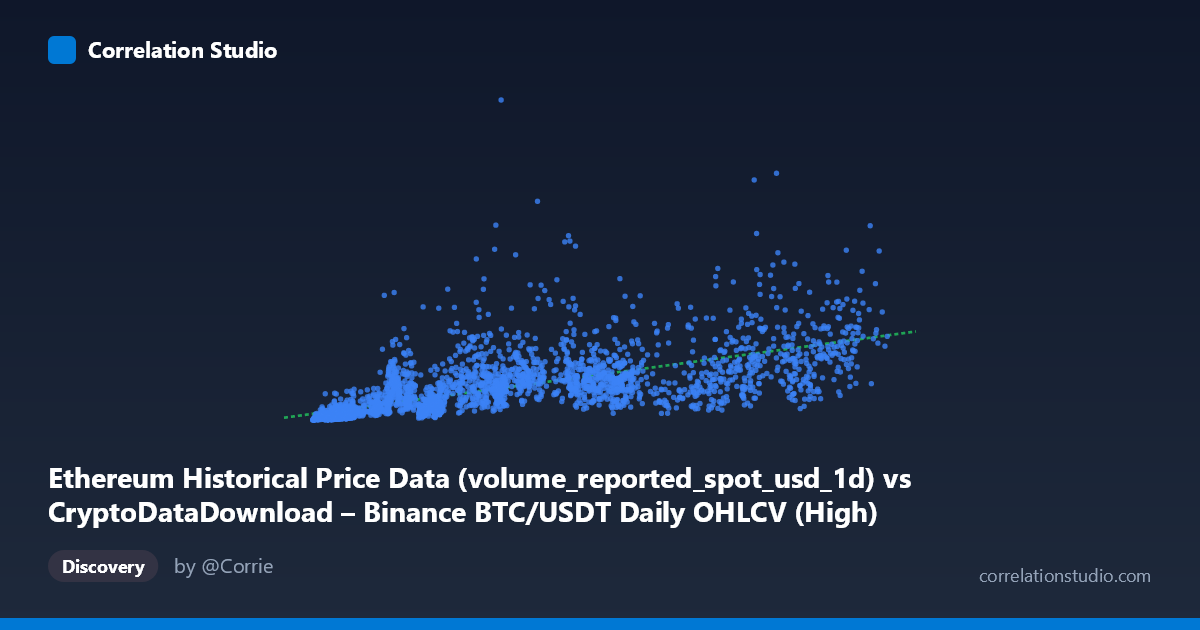
Ethereum Historical Price Data (volume_reported_spot_usd_1d) vs CryptoDataDownload – Binance BTC/USDT Daily OHLCV (High)
- Pearson correlation (r)
- 0.682
- Spearman correlation
- 0.8461
- p-value
- 0
- Sample size (n)
- 3191
- 95% confidence interval
- 0.663 to 0.7001
- Granger causality
- Y → X
- Granger optimal lag
- 10
- Time coverage
- 2017-08-17 to 2026-05-20
AI analysis
Analysis: Trading Volume vs. Price Relationship
1. What the Visualization Reveals
Despite the confusing column labels (the data appears to actually represent trading volume on the X-axis and price/volume metrics on the Y-axis, likely mislabeled in the source), the scatterplot shows a moderate positive relationship between the two variables. As X increases, Y tends to increase as well, but with substantial scatter around the trend line, especially at higher X values. The relationship shows signs of heteroscedasticity — the spread of Y values widens considerably as X grows, which is typical of financial/volume data spanning multiple orders of magnitude.
2. Strength, Direction, and Statistical Significance
The correlation coefficient (r = 0.682) indicates a moderate-to-strong positive linear relationship, but r² = 0.465 tells the more important story: only 46.5% of the variance in Y is explained by X, leaving more than half unexplained by this single variable. The 95% CI [0.663, 0.700] is tight given the large sample size (n=3,191), and the p-value of ~0 confirms this correlation is highly statistically significant — it is not due to chance. However, statistical significance should not be conflated with practical predictive power; a moderate r² means X alone is an incomplete model for Y.
The Granger causality results add a critical temporal dimension: Y Granger-causes X, not the reverse (F=2.43, p=0.0069 for Y→X vs. F=1.24, p=0.258 for X→Y). This suggests that past values of Y contain predictive information about future values of X at a 10-period lag, but not vice versa. This is an important asymmetry — the correlation is contemporaneous/associative, but the predictive direction runs from Y to X, which has implications for any forecasting model built on this data.
3. Notable Patterns and Outliers
Several data points stand out: at X≈41,100, Y jumps to ~$14.6B, and at X≈56,758, Y reaches ~$13.7B — both well above the regression line, suggesting volume/price spikes possibly tied to specific market events (news, liquidations, exchange listings). Conversely, many low-X points cluster tightly near the origin with small Y values, indicating a floor effect at low volume/price levels. The Spearman ρ exceeding Pearson r is a meaningful diagnostic — it indicates the relationship is monotonic but not well captured by a straight line, pointing to a logarithmic, power-law, or polynomial relationship more consistent with typical volume-price dynamics in crypto markets (where relationships often compress or expand multiplicatively rather than additively).
4. Confounding Factors and Caveats
The metadata reveals a likely data pipeline error: X is labeled as Ethereum volume data but pulled from a "Binance BTC/USDT" column, and Y is labeled as BTC/USDT High price but sourced from an "Ethereum" dataset. This cross-contamination between BTC and ETH data raises serious concerns about what relationship is actually being measured — it may reflect general crypto market co-movement (both assets tend to rise/fall together) rather than a genuine causal or mechanical link between volume and price. Additionally, the ~9-year time span (2017–2026) means both series are non-stationary trending series (increasing prices, changing volume regimes across bull/bear cycles), which can produce spurious correlations and inflate both r and Granger causality statistics if not properly detrended.
5. Actionable Insights
1. Verify column mapping — confirm whether this is truly BTC volume vs. ETH price, or a mislabeled BTC-only relationship, before drawing asset-specific conclusions. 2. Test log-transformed variables — given the Spearman/Pearson divergence and heteroscedasticity, refit using log(X) and log(Y), which is standard practice for financial volume/price data and likely to raise r². 3. Check stationarity — run ADF/KPSS tests and consider differencing or returns-based analysis before trusting the Granger causality result, as trending data can produce misleading lead-lag signals. 4. Investigate outlier events — identify the dates behind the high-Y outliers (potential news/liquidation events) to see if they should be treated separately or explain via an event-dummy variable. 5. Expand the model — since X explains only 46.5% of variance, consider multivariate models incorporating additional features (market cap, volatility, order book depth) to improve predictive power.
X dataset: CryptoDataDownload – Binance BTC/USDT Daily OHLCV
Y dataset: Ethereum Historical Price Data
Part of experiment: Bitcoin - CryptoDataDownload – Binance BTC/USDT Daily OHLCV vs Ethereum Historical Price Data