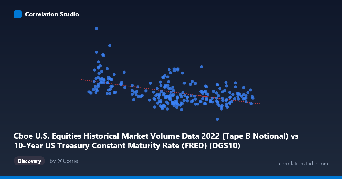
Cboe U.S. Equities Historical Market Volume Data 2022 (Tape B Notional) vs 10-Year US Treasury Constant Maturity Rate (FRED) (DGS10)
- Pearson correlation (r)
- -0.4997
- Spearman correlation
- -0.4471
- p-value
- 0
- Sample size (n)
- 249
- 95% confidence interval
- -0.5875 to -0.4002
- Granger causality
- None
- Granger optimal lag
- 10
AI analysis
Analysis: 10-Year Treasury Yield vs. Cboe Tape B Notional Volume (2022)
Relationship Overview
The scatterplot reveals a moderate negative relationship between the 10-year US Treasury constant maturity rate (X-axis) and Cboe Tape B notional trading volume (Y-axis) across 249 trading days in 2022. The linear regression equation (y = -1.604×10⁹x + 1.211×10¹⁰) indicates that for each one-percentage-point increase in the 10-year yield, notional volume is predicted to decrease by approximately $1.6 billion. This directional pattern is economically intuitive: as interest rates rose aggressively throughout 2022 — from roughly 1.63% to 4.25% — equity market participation as measured by notional volume on Tape B venues (regional exchanges) broadly declined, consistent with risk-off sentiment and portfolio reallocation away from equities toward higher-yielding fixed income instruments.
Correlation Strength and Statistical Significance
The Pearson correlation of r = -0.4997 reflects a moderate negative association, but the explanatory power is meaningfully limited: r² = 0.2497 means only ~25% of the variance in notional volume is explained by the yield level. The remaining 75% of variation stems from other factors entirely uncaptured by this single-variable model. The 95% confidence interval of [-0.5875, -0.4002] is reasonably tight and does not cross zero, and the p-value of effectively 0 confirms this correlation is highly statistically significant given n = 249 and N = 4,769. However, statistical significance here reflects the precision of the estimate rather than practical magnitude — a quarter of variance explained is noteworthy but far from deterministic. Crucially, Granger causality testing finds no significant predictive directionality in either direction (X→Y: F = 1.43, p = 0.168; Y→X: F = 1.10, p = 0.361) at the optimal 10-period lag. This means that while the two series are contemporaneously correlated, neither reliably predicts the other temporally — the correlation likely reflects co-movement driven by shared macro conditions rather than a lead-lag causal mechanism.
Notable Patterns, Clusters, and Outliers
The scatterplot displays considerable vertical dispersion at virtually every yield level, particularly in the 2.8%–3.2% range where notional volume values span roughly $4.2 billion to $11.7 billion — a nearly 3× range for similar yield readings. Several high-volume outliers are visible at lower yield levels (e.g., ~$14.8B at 1.75%, ~$14.2B at 1.86%, ~$12.3B at 1.81%), likely corresponding to high-volatility sessions in early 2022 when rate uncertainty was spiking and equity turnover surged. There also appears to be a non-linear or heteroscedastic pattern: variance in volume is substantially higher at low yields (1.6%–2.2%) than at higher yields (3.5%–4.25%), where volume clusters more tightly in a lower range. This funnel-shaped dispersion suggests the linear model may underfit the lower yield regime and that a polynomial or piecewise regression could better capture the structural relationship.
Confounding Factors and Interpretation Caveats
Several important caveats complicate causal interpretation. First, 2022 was an exceptional macro year — the Federal Reserve executed its fastest rate-hiking cycle in decades, and both variables were simultaneously driven by the same underlying inflation and monetary policy shock, making it difficult to disentangle direct rate effects on volume from shared confounders. Second, Tape B specifically captures regional exchange volume, which may respond differently to rate environments than consolidated market volume; this sub-segment may reflect market microstructure dynamics (e.g., routing changes, maker-taker fee adjustments) that have little to do with rate levels. Third, day-of-week effects, options expiration cycles, index rebalancing events, and geopolitical shocks (e.g., Russia-Ukraine conflict escalation) likely contributed substantial idiosyncratic variance. Fourth, the absence of Granger causality is a meaningful caution against any trading strategy that would attempt to use rate movements to predict near-term volume changes or vice versa.
Actionable Insights and Further Investigation
Practitioners and researchers should pursue several follow-on analyses. Regime segmentation — splitting the sample into Fed hiking sub-periods (e.g., pre/post first hike in March 2022) — could reveal whether the correlation structure changed as the hiking cycle matured and markets adapted. Multivariate modeling incorporating VIX, overall market returns, and broader equity volume (Tapes A and C) would likely substantially improve explanatory power beyond the current 25%. Given the heteroscedastic appearance of the data, a log transformation of the Y variable or robust regression methods would be worth testing to stabilize variance and potentially reveal a cleaner underlying relationship. Finally, repeating this analysis across multiple years (2018–2024) would help determine whether this negative correlation is a structural feature of the rate-volume relationship or a 2022-specific artifact of an unprecedented policy shock.
X dataset: 10-Year US Treasury Constant Maturity Rate (FRED)
Y dataset: Cboe U.S. Equities Historical Market Volume Data 2022
Part of experiment: Daily - 10-Year US Treasury Constant Maturity Rate (FRED) vs Cboe U.S. Equities Historical Market Volume Data 2022