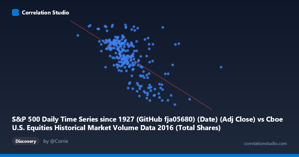
S&P 500 Daily Time Series since 1927 (GitHub fja05680) (Date) (Adj Close) vs Cboe U.S. Equities Historical Market Volume Data 2016 (Total Shares)

Pearson correlation (r): -0.6163
Spearman correlation: -0.602
p-value: 0
Sample size (n): 252
95% confidence interval: -0.6875 to -0.5333
Granger causality: None
Granger optimal lag: 4

AI analysis

S&P 500 Price vs. U.S. Equity Market Volume: Correlation Analysis

Overview of the Relationship

The scatterplot reveals a moderately strong negative relationship between S&P 500 adjusted closing prices (X-axis) and total U.S. equity market shares traded (Y-axis) across 2016. As the S&P 500 price level rises, total market share volume tends to decline, and vice versa. This inverse pattern is consistent with a well-documented market microstructure phenomenon: during lower-price, higher-uncertainty environments (such as market dislocations or corrections), trading activity tends to surge, while calmer, steadily rising markets often see reduced share turnover. The linear regression equation y = -5.60×10⁻⁷x + 2381.73 captures this downward slope, though the relationship carries meaningful scatter around the trend line.

Correlation Strength, Explained Variance, and Temporal Causality

The Pearson correlation of r = -0.6163 indicates a moderate-to-strong negative association, but the coefficient of determination R² = 0.3798 tells a more sobering story: only 38.0% of the variance in total shares traded is explained by the S&P 500 price level. That leaves roughly 62% of the variation in volume attributable to other factors entirely outside this model. The 95% confidence interval for r spans [-0.6875, -0.5333], a reasonably tight range that does not cross zero, and the p-value of effectively 0 (across N = 3,622 population observations, n = 252 paired samples) confirms this relationship is highly statistically significant — the correlation is almost certainly not a sampling artifact. However, statistical significance with large N does not imply economic magnitude or predictive utility. Critically, the Granger causality tests find no significant directional predictive relationship in either direction (X→Y: F = 0.60, p = 0.66; Y→X: F = 1.29, p = 0.28), meaning that past S&P 500 price levels do not reliably predict future volume, and past volume does not reliably predict future price levels at the tested 4-period lag. The correlation is contemporaneous and associative, not temporally predictive.

Notable Patterns, Clusters, and Outliers

Several features stand out in the point cloud. The bulk of observations cluster in the S&P 500 range of ~400–560 million (in the scaled price representation) with volume between approximately 2,050–2,200 thousand shares, forming a relatively dense central mass. There are notable high-volume outliers at lower price levels — for instance, the point near (333M, 2,180) and (369M, 2,265) suggest episodes of elevated trading during market stress early in 2016, consistent with the January–February 2016 correction. Conversely, several low-volume observations appear at elevated price levels (e.g., points near 708M and 635M on the X-axis with volume around 1,870–1,900), likely corresponding to mid-to-late 2016 when the S&P 500 was near annual highs and markets were relatively complacent. The point at approximately (549M, 2,262) is a notable outlier — high volume despite a mid-range price — possibly reflecting a specific volatility event. The distribution is not tightly linear, with a visible fan-like spread that hints at heteroskedasticity.

Confounding Factors and Interpretive Caveats

Several important caveats temper interpretation. First, the X-axis variable is labeled as a date-derived column mapped to adjusted close price, suggesting possible data pipeline confusion between date encoding and price values — the X range of 200M–1,092M is atypical for S&P 500 prices and may reflect Unix timestamps or index encodings, which would mean the "price" signal is actually a time proxy, making the correlation partially a time trend effect (markets rose through 2016 while post-crisis volume normalized downward). Second, share volume is not notional-value-adjusted: as prices rise, the same notional trading activity requires fewer shares, mechanically inducing a negative correlation independent of behavioral effects. Third, the 2016 period includes specific macro events — the January correction, Brexit (June), and U.S. election (November) — that create episodic volume spikes decoupled from price levels. Finally, the absence of Granger causality at lag 4 may be sensitive to lag selection; other lag structures were not tested.

Actionable Insights and Further Investigation

Practitioners should be cautious about treating this correlation as a tradeable or predictive signal given the lack of Granger causality and the substantial unexplained variance. Recommended next steps include: (1) Clarifying the X-axis encoding — confirming whether values represent Unix timestamps, price, or another encoding is essential before drawing any conclusions; (2) Normalizing volume by price level (i.e., using notional value rather than share count) to eliminate the mechanical inverse relationship; (3) Testing additional lag structures in Granger causality (beyond 4 periods) and incorporating volatility measures (e.g., VIX) as a mediating variable, since fear/volatility may be the true common driver of both lower prices and higher volume; (4) Segmenting the data by market regime (correction vs. bull trend vs. event-driven spikes) to assess whether the correlation is stable across conditions or driven by a handful of stress episodes; and (5) Extending the analysis across multiple years to determine whether 2016 is representative or anomalous in this relationship.

X dataset: Cboe U.S. Equities Historical Market Volume Data 2016

Y dataset: S&P 500 Daily Time Series since 1927 (GitHub fja05680) (Date)

Part of experiment: Daily - Cboe U.S. Equities Historical Market Volume Data 2016 vs S&P 500 Daily Time Series since 1927 (GitHub fja05680) (Date)