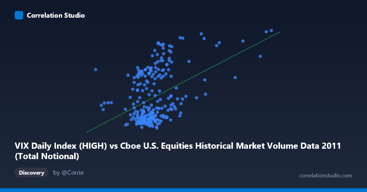
VIX Daily Index (HIGH) vs Cboe U.S. Equities Historical Market Volume Data 2011 (Total Notional)
- Pearson correlation (r)
- 0.447
- Spearman correlation
- 0.3716
- p-value
- 0
- Sample size (n)
- 252
- 95% confidence interval
- 0.3424 to 0.5407
- Granger causality
- None
- Granger optimal lag
- 1
AI analysis
Scatterplot Analysis: VIX Daily Index (HIGH) vs. Total Notional Market Volume (2011)
Relationship Overview
The scatterplot reveals a moderate positive relationship between the VIX Daily Index High values and the Total Notional trading volume in U.S. equities markets during 2011. As VIX high readings increase, there is a general tendency for total notional volume to rise as well, consistent with the well-established financial intuition that elevated market fear and uncertainty — as captured by the VIX — tends to drive higher trading activity. The linear regression equation (y = 9.64×10⁻¹⁰x + 9.12) indicates a positive slope, though the relationship is clearly noisy, with considerable vertical spread at most VIX levels, suggesting the association is real but far from deterministic.
Correlation Strength and Statistical Significance
The Pearson correlation of r = 0.447 indicates a moderate positive association, but the explanatory power is modest: r² = 0.20, meaning only about 20% of the variance in total notional volume is explained by VIX high readings. The remaining 80% is driven by other factors entirely. The 95% confidence interval for r of [0.342, 0.541] is reasonably tight, reflecting the solid sample size (n = 252), and the p-value of 8.77×10⁻¹⁴ confirms this correlation is highly statistically significant and extremely unlikely to be a chance finding. However, statistical significance here should be interpreted cautiously — with N = 3,780 as the broader population context, even modest correlations can achieve significance. More importantly, Granger causality tests in both directions are non-significant (X→Y: p = 0.687; Y→X: p = 0.991), meaning neither variable temporally predicts the other at the optimal lag of 1 period. This is a critical nuance: while the variables co-move, there is no detectable predictive temporal precedence in either direction, strongly suggesting the relationship is contemporaneous and likely driven by common underlying factors rather than a causal chain.
Notable Patterns, Clusters, and Outliers
The data exhibits several visually distinct features. A dense cluster of points appears at lower VIX levels (roughly 14–22) paired with lower notional volumes (approximately 13–18 billion), forming a tight concentration that anchors the lower-left region of the plot. Above VIX levels of approximately 25–30, the vertical spread widens dramatically, indicating increased heteroscedasticity — volume becomes far more variable as volatility rises. Several notable outliers appear in the upper regions: data points with VIX highs above 35–40 (consistent with the 2011 U.S. debt ceiling crisis and European sovereign debt turmoil in mid-to-late summer) show exceptionally high notional volumes, including readings near 42–48 on the Y-axis paired with volumes in the 26–38 billion range. These extreme observations likely exert significant leverage on the regression line and may be driving much of the observed correlation.
Confounding Factors and Caveats
Several important caveats apply to this analysis. First, 2011 was an atypical year characterized by the U.S. debt ceiling standoff, the S&P downgrade of U.S. sovereign debt, and the European debt crisis — all of which produced episodic spikes in both VIX and trading volume simultaneously, potentially inflating the observed correlation relative to more typical market periods. Second, market structure factors such as end-of-quarter rebalancing, options expiration dates, and index reconstitution events independently drive volume surges regardless of volatility levels, acting as confounders. Third, the heteroscedasticity visible in the plot violates a core assumption of linear regression, suggesting the linear model may be misspecified and that a log-transformed or quantile regression approach might be more appropriate. Finally, the axes appear to be swapped relative to the dataset labels (VIX is plotted on X, notional volume on Y), which is worth confirming against the raw data structure.
Actionable Insights and Further Investigation
Despite the non-causal Granger result, the moderate correlation and the clustering patterns offer practical value. Risk managers and trading desks could use VIX levels as a contemporaneous signal for expected volume regimes, even if VIX cannot predict volume one day ahead. To deepen this analysis, it would be worthwhile to: (1) segment the data by VIX regime (e.g., low: <20, elevated: 20–30, crisis: 30) to examine whether the correlation strengthens materially in high-volatility periods; (2) apply a log-log regression to address heteroscedasticity and potentially reveal a stronger power-law relationship; (3) incorporate additional lagged variables such as S&P 500 returns, bid-ask spreads, or overnight futures moves to build a more complete explanatory model; and (4) replicate the analysis across multiple years to determine whether the 2011 correlation is anomalously high due to crisis conditions or representative of a stable structural relationship.
X dataset: Cboe U.S. Equities Historical Market Volume Data 2011
Y dataset: VIX Daily Index
Part of experiment: Daily - Cboe U.S. Equities Historical Market Volume Data 2011 vs VIX Daily Index