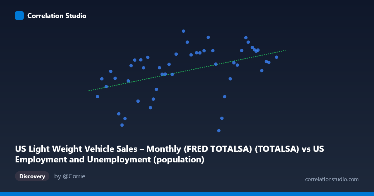
US Light Weight Vehicle Sales – Monthly (FRED TOTALSA) (TOTALSA) vs US Employment and Unemployment (population)
- Pearson correlation (r)
- 0.4479
- Spearman correlation
- 0.5301
- p-value
- 0.001109
- Sample size (n)
- 50
- 95% confidence interval
- 0.1936 to 0.6457
- Granger causality
- None
- Granger optimal lag
- 1
- Time coverage
- 1976-01-01 to 2025-01-01
- Recomputed on refreshed data
- 2026-10-07 (r was 0.4295)
AI analysis
Scatterplot Analysis: US Light Vehicle Sales vs. US Population
Overall Relationship
The scatterplot reveals a modest positive relationship between US light-weight vehicle sales (X-axis, measured in millions of units SAAR) and US population (Y-axis, in tens of millions). The linear regression equation y = 2.66×10⁻⁵x + 9.38 captures an upward trend, suggesting that as vehicle sales volumes increase, they tend to occur during periods of larger population. This makes intuitive sense across a nearly 50-year span (1976–2025), as both variables share a common driver: long-run demographic and economic growth. However, the relationship is far from tight, and considerable scatter is visible throughout the plot.
Correlation Strength and Statistical Significance
The correlation of r = 0.43 is statistically significant (p = 0.0019, well below the 0.05 threshold), but the practical magnitude is modest. The R² = 0.185 tells the more sobering story — only 18.5% of the variance in population is explained by vehicle sales, leaving over 80% attributable to other factors. The 95% confidence interval [0.17, 0.63] is notably wide, spanning from weak to moderately strong correlation, which reflects meaningful uncertainty given the sample of n = 50. Critically, Granger causality tests show no significant predictive direction in either direction (X→Y: F = 0.65, p = 0.42; Y→X: F = 0.87, p = 0.35). This means vehicle sales do not temporally predict population changes, nor vice versa — the observed correlation likely reflects a shared secular trend rather than any causal mechanism.
Notable Patterns, Clusters, and Outliers
Several features stand out in the scatterplot. There is a loose central cluster of points around X ≈ 200,000–230,000 and Y ≈ 14–17, consistent with the sample means. However, notable outliers disrupt the trend: - (172,271; 10.29) and (174,215; 10.87) — low sales AND low population, consistent with early dataset years (late 1970s/early 1980s) - (235,801; 9.79) — the lowest Y value paired with mid-to-high X, a clear outlier that pulls against the trend - (237,830; 10.89) — similarly anomalous, suggesting a period where sales were high but population metrics appear suppressed, possibly a data alignment issue - (212,577; 18.64) — the highest Y value at mid-range X, suggesting population-era peaks don't align with maximum sales
The non-linearity is also notable: at higher X values (240,000), Y values scatter widely between ~10 and 18, suggesting the relationship weakens or reverses at extremes.
Confounding Factors and Caveats
Several important caveats apply. First, both variables trend upward over time, meaning the correlation may be largely spurious co-trending — a classic pitfall in long time-series analysis. Second, the dataset mismatch is significant: vehicle sales are monthly (SAAR), while population/employment data are annual — temporal aggregation and alignment introduce noise. Third, economic cycles (recessions in 1981, 2001, 2008–09, 2020) create episodic crashes in vehicle sales that don't mirror population patterns, explaining much of the scatter. Fourth, the outlier at (235,801; 9.79) warrants scrutiny — it may reflect a data entry error, misaligned join, or structural break in one of the series. The wide confidence interval further cautions against over-interpreting the r value.
Actionable Insights and Further Investigation
Given the weak explanatory power and absent Granger causality, vehicle sales should not be modeled as a predictor of population (or vice versa) in any direct sense. However, both likely respond to common third variables. Recommended next steps include: (1) detrending both series (e.g., first-differencing or HP filter) before re-examining correlation, to isolate cyclical co-movement from shared trends; (2) investigating the apparent outliers — particularly the (235,801; 9.79) point — to verify data integrity; (3) introducing mediating variables such as GDP, unemployment rate, consumer sentiment, or interest rates, which plausibly drive both population-linked demand and auto sales simultaneously; and (4) segmenting the analysis by decade to test whether the correlation is stable across economic regimes or driven entirely by a specific era. A VAR model with proper controls would yield far richer causal insight than bivariate correlation alone.
X dataset: US Employment and Unemployment
Y dataset: US Light Weight Vehicle Sales – Monthly (FRED TOTALSA)
Part of experiment: Yearly - US Employment and Unemployment vs US Light Weight Vehicle Sales – Monthly (FRED TOTALSA)