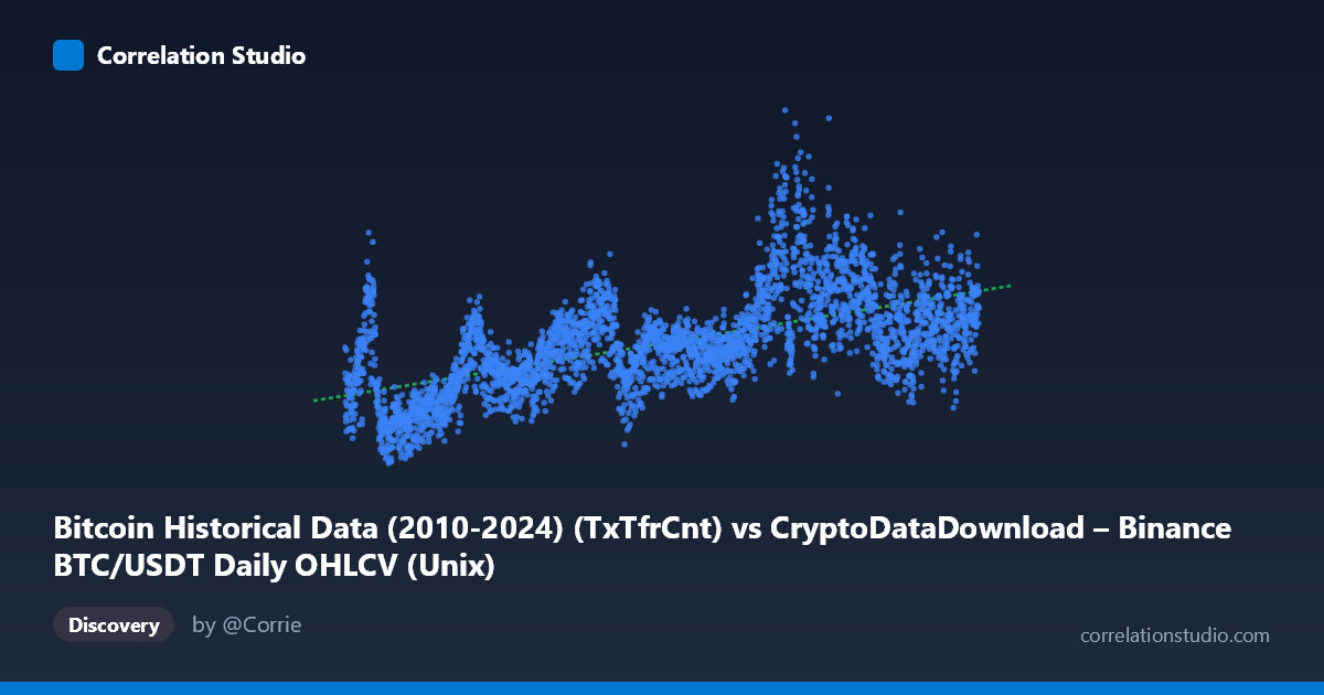
Bitcoin Historical Data (2010-2024) (TxTfrCnt) vs CryptoDataDownload – Binance BTC/USDT Daily OHLCV (Unix)
- Pearson correlation (r)
- 0.6
- Spearman correlation
- 0.6278
- p-value
- 0
- Sample size (n)
- 3191
- 95% confidence interval
- 0.5774 to 0.6218
- Granger causality
- None
- Granger optimal lag
- 10
AI analysis
Analysis: Bitcoin Timestamp vs. Transaction Count Relationship
1. What the Visualization Reveals
The scatterplot depicts a moderate positive relationship between a Unix timestamp (X, effectively "time") and Bitcoin transaction count (Y), spanning nearly a decade (2017–2026) of daily data. Since X is essentially a linear proxy for calendar time, this chart is fundamentally showing how transaction counts have trended upward over the life of the dataset, albeit with substantial scatter around that trend. The relationship is far from a clean line — Y values at similar X points range widely (e.g., in 2024, values span from ~837K to ~1.38M), indicating that time alone is a weak-to-moderate predictor of transaction activity on any given day.
2. Strength, Direction, and Statistical Confidence
The correlation coefficient (r = 0.60) indicates a moderate positive relationship, with the tight 95% CI [0.577, 0.622] and p-value of 0 confirming this estimate is highly reliable given the large sample (n=3,191) — there's essentially no doubt a real, non-zero association exists. However, r² = 0.36 tells the more practically important story: only 36% of the variance in transaction count is explained by time, leaving 64% attributable to other factors (market cycles, adoption waves, network congestion events, fee dynamics, etc.). Critically, the Granger causality tests show no significant predictive direction in either direction (X→Y: p=0.080; Y→X: p=0.752) at the optimal lag of 10 periods. This is an important caveat: since X is just a timestamp, Granger causality is somewhat conceptually odd here (time cannot be "caused" by transaction count), but the near-significant X→Y result (p=0.08) hints that past temporal position has weak marginal predictive value for future transaction counts beyond autocorrelation — not a strong basis for forecasting.
3. Notable Patterns and Non-Linear Features
The data suggests a non-monotonic, cyclical trend rather than steady linear growth — consistent with Bitcoin's known boom-bust cycles. Sample points show low transaction counts in 2017-2018 (~370K–670K), a rise through 2020-2021 (~850K-1.2M with a spike to 1.18M-1.21M around late 2023/2024), and continued volatility through 2024-2026 without clear stabilization. This suggests the true relationship may be better modeled by piecewise segments or cyclical/seasonal components tied to bull/bear markets rather than a single linear fit. The linear R² of 0.36 likely understates fit quality during trending sub-periods and overstates it during consolidation periods — visual inspection likely shows fan-shaped or wave-like clustering rather than a uniform band around the regression line.
4. Confounding Factors and Caveats
Several concerns limit causal interpretation: (1) Spurious trend correlation — two variables that both trend over time (even for unrelated reasons) will show positive correlation; this is a classic time-series confound. (2) Omitted variables: price volatility, exchange volume, network fee levels, regulatory events, and macro liquidity conditions likely drive transaction counts far more directly than "time" itself. (3) Autocorrelation: daily transaction counts are highly autocorrelated, meaning standard r/p-value calculations (assuming independent observations) may overstate statistical confidence — effective sample size is likely much smaller than 3,191. (4) The dataset description mismatch (X labeled as "TxTfrCnt" but described as timestamp-like, Y labeled as Unix timestamp but behaving like transaction count) suggests possible column mislabeling that should be verified before drawing firm conclusions.
5. Actionable Insights and Further Investigation
Given the weak causality signal and time-driven confound, time alone should not be used as a standalone predictor of transaction counts. Instead: (a) decompose the series into trend/seasonal/cyclical components (e.g., STL decomposition) to isolate genuine drivers from calendar drift; (b) test correlation against more direct covariates — BTC price, trading volume, or realized volatility — which likely explain more variance; (c) apply differencing or detrending before rerunning correlation/Granger tests to address non-stationarity and autocorrelation inflation; and (d) verify column definitions/data lineage given the apparent axis-label confusion, as this affects interpretation validity. A regime-based analysis (splitting by bull/bear market phases) would likely reveal much stronger localized correlations than the pooled 0.60 figure suggests.
X dataset: CryptoDataDownload – Binance BTC/USDT Daily OHLCV
Y dataset: Bitcoin Historical Data (2010-2024)
Part of experiment: Bitcoin - CryptoDataDownload – Binance BTC/USDT Daily OHLCV vs Bitcoin Historical Data (2010-2024)