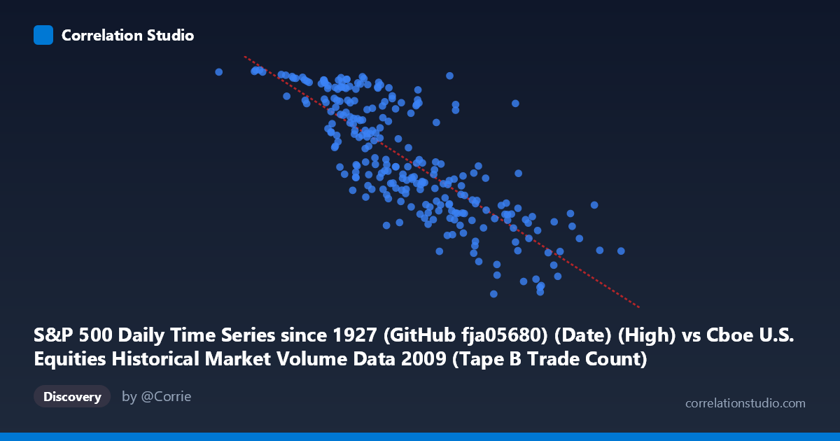
S&P 500 Daily Time Series since 1927 (GitHub fja05680) (Date) (High) vs Cboe U.S. Equities Historical Market Volume Data 2009 (Tape B Trade Count)
- Pearson correlation (r)
- -0.8013
- Spearman correlation
- -0.8148
- p-value
- 0
- Sample size (n)
- 252
- 95% confidence interval
- -0.8416 to -0.7522
- Granger causality
- Bidirectional
- Granger optimal lag
- 10
AI analysis
Analysis: S&P 500 Daily High vs. Cboe Tape B Trade Count (2009)
Relationship Overview The scatterplot reveals a clear negative relationship between the S&P 500 daily high price (X-axis) and the Cboe Tape B trade count (Y-axis) across 2009 trading days. As the index moved to higher price levels, the number of Tape B trades declined substantially — a pattern consistent with the market's recovery arc during 2009, where the index climbed from post-crisis lows in early spring toward year-end highs while trading volume and activity gradually normalized downward from panic-driven extremes. The linear regression equation (y = −0.000725x + 1,247.79) captures this inverse trajectory, though the relationship carries meaningful financial interpretation beyond mere arithmetic.
Correlation Strength and Statistical Robustness The correlation of r = −0.80 is strong and statistically unambiguous (p ≈ 0, n = 252). The r² = 0.6421 indicates that roughly 64% of the variance in Tape B trade counts is explained by the S&P 500 daily high — a substantial explanatory share, though it also means ~36% of variation is driven by other factors. The 95% confidence interval of [−0.84, −0.75] is tight and entirely negative, leaving no credible room for a null or positive relationship. The Granger causality results are particularly notable: both directions are statistically significant at the 10-period lag (X→Y: F=2.21, p=0.018; Y→X: F=2.19, p=0.019), indicating bidirectional temporal predictability. This means neither variable is cleanly "causal" — past S&P highs help predict future trade counts, but past trade counts also help predict future index highs, likely reflecting the deeply co-integrated nature of price discovery and market participation during a volatile recovery year.
Patterns, Clusters, and Outliers The sample points reveal a roughly linear but somewhat heteroscedastic cloud — variance in trade counts is visibly wider at lower index values (roughly 81,000–300,000 range), where several high-count observations cluster (e.g., the point near x=81,703, y=1,126 and x=156,192, y=1,126). These likely correspond to early 2009 crisis-period sessions when the market was near lows but trading activity was frenetic. At higher index values (500,000–766,000), the points compress into a tighter, lower-activity band (700–900 range), consistent with calmer, trending market conditions in Q3–Q4 2009. One notable outlier is the point at approximately (766,764; 779) — the highest X value with relatively suppressed trade count — possibly a late-year low-volatility session. The two nearly identical X-values around 418,600 but with Y-values of 910 and 1,063 respectively suggest intraday regime differences at similar price levels.
Confounding Factors and Interpretive Caveats This correlation is almost certainly driven substantially by time as a latent variable — 2009 followed a chronological path from market lows (high fear, high volume) to market recovery (lower fear, lower volume), meaning both variables are co-moving with the same underlying temporal trend rather than directly causing each other. The Granger bidirectionality reinforces this: what looks like predictive power may partly reflect shared dependence on macroeconomic recovery dynamics, Fed policy shifts, or VIX normalization. Additionally, Tape B specifically covers NYSE American and regional exchanges, so trade count reflects a subset of total market activity that may be disproportionately affected by retail or smaller-cap trading behavior. The dataset's N=3,232 suggests the full population is much larger than the 252-day sample, and aggregation at the daily level masks intraday structure that could alter interpretations significantly.
Actionable Insights and Further Investigation Given the bidirectional Granger causality, a practitioner could reasonably explore Tape B trade count as a leading or coincident sentiment indicator for near-term index direction — elevated trade counts at lower prices may signal capitulation bottoms worth monitoring. Further investigation should include: (1) decomposing the time trend via detrended residual analysis to isolate whether any relationship persists beyond the shared 2009 recovery arc; (2) comparing Tape A and Tape C trade counts to determine whether this inverse pattern is exchange-specific or market-wide; (3) incorporating VIX or bid-ask spread data as mediating variables to test whether volatility explains the volume-price divergence more directly; and (4) extending the analysis across multiple years (2008, 2010) to assess whether this negative correlation is structurally persistent or unique to crisis-recovery regimes. The 64% explained variance is compelling but should not support trading strategies without controlling for the temporal confound.
X dataset: Cboe U.S. Equities Historical Market Volume Data 2009
Y dataset: S&P 500 Daily Time Series since 1927 (GitHub fja05680) (Date)
Part of experiment: Daily - Cboe U.S. Equities Historical Market Volume Data 2009 vs S&P 500 Daily Time Series since 1927 (GitHub fja05680) (Date)