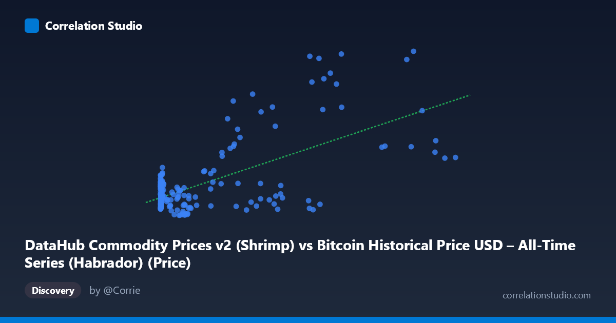
DataHub Commodity Prices v2 (Shrimp) vs Bitcoin Historical Price USD – All-Time Series (Habrador) (Price)
- Pearson correlation (r)
- 0.6445
- Spearman correlation
- 0.2868
- p-value
- 0
- Sample size (n)
- 182
- 95% confidence interval
- 0.5507 to 0.7223
- Granger causality
- None
- Granger optimal lag
- 1
- Time coverage
- 2010-08-01 to 2025-09-01
AI analysis
Analysis: Bitcoin Price vs. Shrimp Commodity Price
1. What the Visualization Reveals
The scatterplot shows a moderate positive relationship between Bitcoin's historical USD price (X-axis) and a shrimp commodity price index (Y-axis). Most data points cluster in the lower-left region, where Bitcoin prices are below ~10,000 and shrimp prices stay within a tight band of roughly 1.0–2.0. As Bitcoin prices climb into the tens of thousands, the Y-values become more dispersed, with several points spiking to 2.5–5.1 — suggesting the relationship is not uniform across the full range of X.
2. Strength, Direction, and Uncertainty
The correlation coefficient (r = 0.6445) indicates a moderate positive linear association, but r² = 0.4154 tells the more important story: only about 41.5% of the variance in shrimp prices is explained by Bitcoin price, leaving the majority (58.5%) driven by other factors. The 95% CI [0.55, 0.72] is reasonably tight and excludes zero, and the p-value of ~0 confirms this correlation is statistically robust, not a chance artifact of sampling.
However, the Granger causality results are critical for interpretation: neither variable significantly predicts the other (X→Y: p=0.742; Y→X: p=0.406). This strongly suggests the correlation is not causal in either direction — it's more likely that both series are trending upward over the same 2010–2025 time window (Bitcoin due to adoption/speculation, shrimp prices due to inflation/commodity cycles) rather than one driving the other. This is a classic case of spurious correlation via shared time trend.
3. Notable Patterns and Outliers
Several notable features stand out: - Nonlinear/heteroscedastic spread: Variance in Y increases dramatically as X increases (fanning pattern), violating a key assumption of simple linear regression. - High-leverage outliers: Points like (97365, 5.10), (105620, 2.56), and (27983.75, 3.85) sit far above the regression line and appear to disproportionately drive the correlation — likely corresponding to 2021 and 2024–2025 Bitcoin bull runs coinciding with commodity/inflation spikes. - Dense low-X cluster: The bulk of points with X < 5,000 show shrimp prices confined to 1.0–1.7, with weak internal correlation — the "relationship" is largely an artifact of a handful of high-X, high-Y observations.
4. Confounding Factors and Caveats
The most obvious confound is time itself. Both Bitcoin and commodity prices have risen over 2010–2025 due to macroeconomic factors (inflation, USD devaluation, global monetary policy, post-pandemic supply chain effects) rather than any direct economic link between cryptocurrency speculation and shrimp markets. Additional caveats: - The Granger test's failure to find lead-lag structure reinforces that this is likely a common-trend/confounding scenario rather than genuine predictive coupling. - Bitcoin's extreme volatility and skewed distribution (mean 17,943 vs. range up to 113,500) means a few large-X points have outsized leverage on the linear fit. - No detrending or differencing was applied — regressing two non-stationary trending series is a well-known source of spurious high-r² results.
5. Recommendations for Further Investigation
To validate whether any real relationship exists, analysts should: (1) detrend or difference both series (e.g., use % changes or log-returns) and re-run the correlation — genuine relationships should survive this transformation; (2) test for cointegration rather than relying on simple Granger causality on levels; (3) exclude or separately analyze the extreme bull-market outliers to see if the correlation holds in the bulk of the data; and (4) introduce a common macro variable (e.g., CPI, USD index) as a control to check whether it explains the shared trend better than any direct link between the two assets. Absent such analysis, this correlation should be treated as descriptive, not causal or predictive.
X dataset: Bitcoin Historical Price USD – All-Time Series (Habrador)
Y dataset: DataHub Commodity Prices v2
Part of experiment: Bitcoin - Bitcoin Historical Price USD – All-Time Series (Habrador) vs DataHub Commodity Prices v2