DataHub Commodity Prices v2 (Lamb) vs Bitcoin Historical Price USD – All-Time Series (Habrador) (Price)
- Pearson correlation (r)
- 0.7064
- Spearman correlation
- 0.234
- p-value
- 0
- Sample size (n)
- 182
- 95% confidence interval
- 0.6252 to 0.7725
- Granger causality
- None
- Granger optimal lag
- 4
AI analysis
Analysis: Bitcoin Price vs. Lamb Commodity Price
1. Relationship Overview
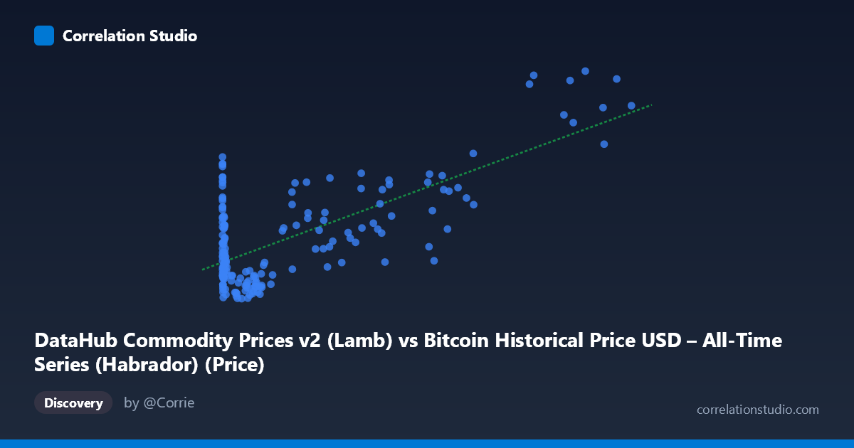
The scatterplot depicts an unusual pairing: Bitcoin's historical USD price (X-axis, spanning genesis through 2025) against a lamb commodity price index (Y-axis). Despite the disparate nature of these series, the data shows a moderate-to-strong positive relationship — as Bitcoin's price rises across its multi-order-of-magnitude range (from fractions of a cent to over $113,500), lamb prices also trend upward, from roughly $120 to over $400. The relationship appears non-linear in raw space (Bitcoin's exponential growth dwarfs lamb's more bounded range), though a linear fit still captures a substantial share of the variance.
2. Strength, Direction, and Statistical Confidence
The correlation coefficient (r = 0.706) indicates a moderately strong positive linear association, with r² = 0.499 meaning essentially half of the variance in lamb prices is statistically explained by Bitcoin price (or vice versa) in this linear model — a substantial but far from complete relationship. The 95% CI [0.625, 0.773] is reasonably tight and excludes zero, and the p-value of ~0 confirms this correlation is highly unlikely to be due to chance in this sample. However, Granger causality tests show no significant predictive direction in either direction (X→Y: p=0.108; Y→X: p=0.363). This is a critical caveat: despite the strong correlation, neither series helps forecast the other's future values based on past patterns. This strongly suggests the relationship is driven by a shared external trend (e.g., both series climbing over the 2010–2025 period due to unrelated macro factors like inflation, dollar depreciation, or simply long-term secular growth) rather than any causal or leading/lagging mechanism.
3. Notable Patterns and Outliers
The data reveals a clear heteroscedastic fan shape: at low Bitcoin prices (under ~$1,000, the majority of early historical points), lamb prices cluster tightly between $120–$250 with high density but wide relative scatter. At high Bitcoin prices ($40,000), lamb prices climb more consistently into the $200–$400+ range, suggesting a possible threshold or regime change rather than a smooth linear relationship throughout. Some early points are notable outliers — e.g., (0.92, 292.07), (3.03, 291.07), and (6.08, 224.16) show very high lamb prices paired with near-zero Bitcoin prices, likely reflecting early Bitcoin history (2010-2011) when lamb prices were already elevated independent of Bitcoin's negligible value. The extreme skew in the X variable (mean 17,943 vs. median likely far lower, given stdev of 27,080) means the regression is heavily influenced by a handful of high-Bitcoin-price observations from recent years.
4. Confounding Factors and Caveats
This pairing raises significant spurious correlation concerns. Both series span 2010–2025, a period of substantial monetary inflation, USD depreciation, and broad asset/commodity price appreciation — any two upward-trending time series over this window will show positive correlation without genuine causal linkage. The mismatch in data granularity (Bitcoin likely daily/high-frequency vs. commodity data "monthly") and the arbitrary sample alignment (every 3rd point shown) may also introduce artifacts. Critically, there's no plausible economic mechanism directly linking Bitcoin valuation to lamb meat pricing — any relationship is almost certainly mediated by common macro drivers (time trend, inflation, global liquidity) rather than direct interaction, which the null Granger causality result reinforces.
5. Actionable Insights
Given the lack of Granger causality, this correlation should not be used for predictive trading or forecasting purposes between these specific assets. Analysts should: (a) detrend both series or test correlation on first-differences/returns rather than levels to check if the relationship persists once the shared time trend is removed (a classic test for spurious correlation); (b) explore whether a shared macro variable (CPI, USD index, or global M2 money supply) explains both trends better than treating them as directly linked; and (c) apply a log transformation to Bitcoin's price (given its exponential growth and range) before re-running correlation/regression to better capture the true functional form and avoid outlier leverage from recent high-price observations.
X dataset: Bitcoin Historical Price USD – All-Time Series (Habrador)
Y dataset: DataHub Commodity Prices v2
Part of experiment: Bitcoin - Bitcoin Historical Price USD – All-Time Series (Habrador) vs DataHub Commodity Prices v2