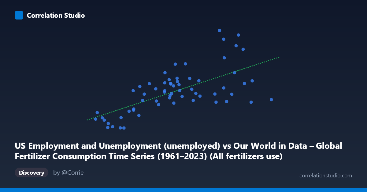
US Employment and Unemployment (unemployed) vs Our World in Data – Global Fertilizer Consumption Time Series (1961–2023) (All fertilizers use)
- Pearson correlation (r)
- 0.6523
- Spearman correlation
- 0.6242
- p-value
- 0
- Sample size (n)
- 63
- 95% confidence interval
- 0.4826 to 0.7749
- Granger causality
- None
- Granger optimal lag
- 10
AI analysis
Analysis of US Unemployment vs. Global Fertilizer Consumption (1961–2023)
1. What the Visualization Reveals
The scatterplot displays a moderately positive relationship between US unemployment (number of unemployed persons, X-axis) and global all-fertilizer consumption (Y-axis) over the period 1961–2023. As unemployment figures rise, fertilizer consumption tends to increase as well. The linear regression equation (y = 0.00036174x + 2,998.76) confirms this upward trend, though the scatter around the regression line is substantial, indicating considerable unexplained variability. Both variables are fundamentally time-driven series — they have both grown over the 62-year observation window — which is a critical interpretive caveat explored below.
2. Correlation Strength, Direction, and Statistical Framing
The Pearson correlation of r = 0.6523 reflects a moderate-to-strong positive association, but the coefficient of determination R² = 0.4255 is the more sobering statistic: only 42.6% of the variance in global fertilizer consumption is explained by US unemployment levels, leaving roughly 57% attributable to other factors. The 95% confidence interval for r [0.4826, 0.7749] is reasonably narrow given the sample size (n = 63), suggesting the true population correlation is unlikely to be trivial, and the p-value of 6.944E-09 confirms the result is highly statistically significant — the probability of observing this correlation by chance alone is vanishingly small. However, statistical significance here is almost certainly inflated by shared secular trends (both series grow over time) rather than any genuine causal mechanism. Critically, the Granger causality tests find no significant predictive directionality in either direction (X→Y: F = 0.718, p = 0.702; Y→X: F = 0.574, p = 0.823), even at an optimal lag of 10 periods. This means that past values of unemployment do not help predict fertilizer consumption beyond its own history, and vice versa — strongly undermining any causal interpretation.
3. Notable Patterns, Clusters, and Outliers
Several features stand out in the data. A lower-left cluster of points (unemployment ~3–6 million, fertilizer use ~2,817–5,156 units) likely corresponds to earlier decades (1960s–1970s) when both series were at lower absolute levels. A middle cluster around unemployment of 10–14 million and fertilizer use of 6,000–9,000 units represents the bulk of the distribution. Several notable outliers deserve attention: (16,970,338; 14,825) and (19,076,803; 14,265) sit well above the regression line, suggesting periods of unusually high fertilizer consumption relative to unemployment; conversely, (22,747,430; 6,314) and (20,491,684; 5,996) fall far below the line — very high unemployment paired with relatively modest fertilizer use — likely corresponding to the COVID-19 pandemic era (2020–2021) when US unemployment spiked dramatically while global fertilizer consumption did not follow proportionally. This divergence at the high-unemployment extreme introduces a non-linear character to the upper range of the distribution.
4. Confounding Factors and Critical Caveats
The most significant caveat is spurious correlation driven by shared time trends. Both US unemployment (in absolute numbers, reflecting population growth and labor force expansion) and global fertilizer consumption have trended upward over six decades due to entirely independent structural forces — population growth, agricultural intensification, and economic expansion. This creates a classic nonsense correlation: two unrelated variables that happen to grow over the same period will appear correlated. The datasets are also conceptually mismatched — one is a US-specific labor market indicator, the other is a global agricultural input metric — and there is no plausible direct causal pathway between them. Additionally, the metadata itself appears to have axis labels swapped (the dataset descriptions suggest X and Y may be mislabeled relative to their source datasets), warranting data verification. Business cycles, global commodity prices, agricultural policy shifts, and technological change in farming are all omitted confounders.
5. Actionable Insights and Further Investigation
Given the absence of Granger causality and the likely spurious nature of the correlation, this relationship should not be used for prediction or policy. Recommended next steps include: (1) detrending both series (e.g., first-differencing or removing polynomial trends) to test whether any correlation persists after removing shared secular growth; (2) cointegration testing (e.g., Engle-Granger or Johansen) to determine if a long-run equilibrium relationship exists beyond coincidental trending; (3) introducing genuine causal candidates such as global GDP, population, energy prices, or agricultural area harvested as covariates in a multivariate model; and (4) verifying axis assignments given the apparent dataset label mismatch. If the goal is understanding fertilizer consumption drivers, analysis should focus on agricultural and economic variables rather than US-specific labor statistics.
X dataset: Our World in Data – Global Fertilizer Consumption Time Series (1961–2023)
Y dataset: US Employment and Unemployment
Part of experiment: Yearly - Our World in Data – Global Fertilizer Consumption Time Series (1961–2023) vs US Employment and Unemployment