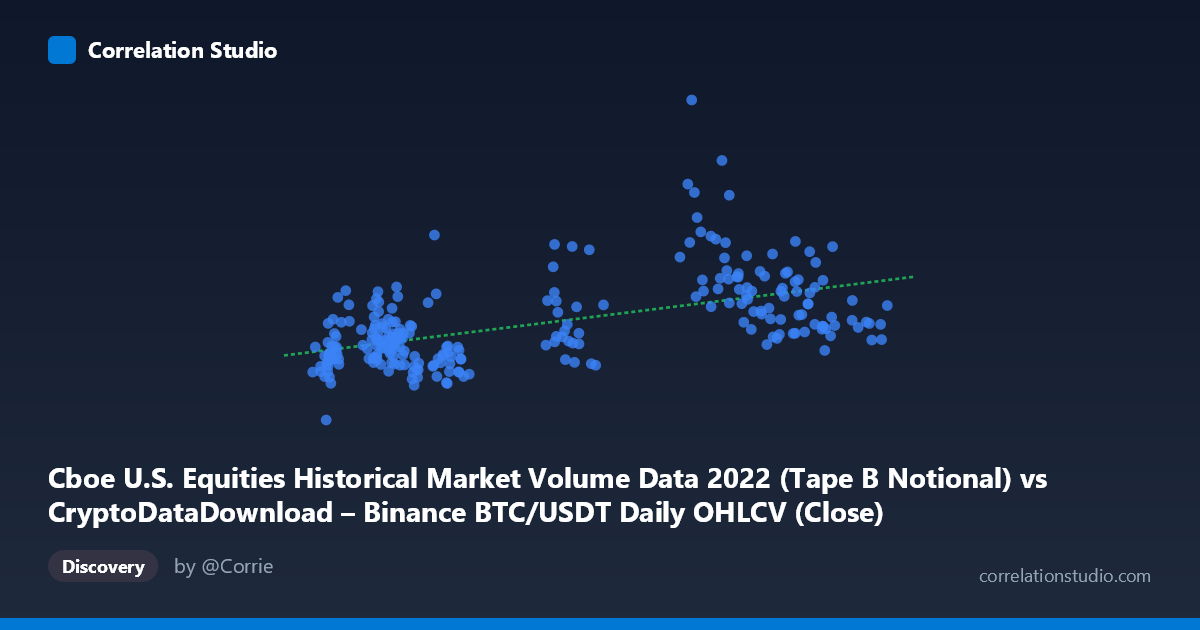
Cboe U.S. Equities Historical Market Volume Data 2022 (Tape B Notional) vs CryptoDataDownload – Binance BTC/USDT Daily OHLCV (Close)

Pearson correlation (r): 0.5418
Spearman correlation: 0.5228
p-value: 0
Sample size (n): 251
95% confidence interval: 0.4481 to 0.6238
Granger causality: None
Granger optimal lag: 10
Time coverage: 2022-01-03 to 2022-12-30

AI analysis

Analysis: Cboe Equity Market Volume vs. BTC/USDT Notional Volume (2022)

Note on axis labeling: The variable names appear swapped in the metadata — X (15,781–47,435 range) is described as Cboe notional volume, while Y (2.2B–19.3B range) is described as BTC/USDT close price. Given the magnitudes, X is more plausibly a BTC-related price/volume metric and Y the equities notional volume in dollars. The analysis below treats the data as presented numerically, but this labeling inconsistency should be resolved before drawing firm conclusions.

1. Overview of the Relationship

The scatterplot shows a moderate positive linear relationship between the two variables. As X increases, Y tends to increase as well, with the fitted regression line (y = 121,282x + 3.94B) sloping upward. However, the relationship is far from tight — there is substantial vertical scatter around the trend line at every X value, indicating that X alone is an incomplete predictor of Y.

2. Strength, Direction, and Statistical Confidence

The correlation coefficient (r = 0.542) indicates a moderate positive association, and r² = 0.294 shows that only ~29% of the variance in Y is explained by X — meaning over 70% of Y's variability stems from other factors. The 95% CI [0.448, 0.624] is reasonably tight and excludes zero, and the p-value (effectively 0) confirms this correlation is highly unlikely to be due to chance at n=251. So while the relationship is statistically robust, it is practically modest — not strong enough for reliable point prediction.

Critically, the Granger causality tests show no significant predictive direction in either direction (X→Y: p=0.398; Y→X: p=0.284). This means that despite the contemporaneous correlation, neither series helps forecast the other's future values based on its own past. This strongly suggests the correlation is driven by a shared external factor (e.g., both series responding to broader 2022 market conditions, volatility regimes, or macro events) rather than one variable causally leading the other.

3. Notable Patterns and Outliers

Several points deviate substantially from the trend, most visibly a cluster with X in the 29,000–39,000 range but unusually high Y values (e.g., 38730.63 → 14.2B, 36445.31 → 14.8B, 36958.32 → 13.0B, 29103.94 → 11.6B). These likely correspond to a specific volatility spike or news-driven event in 2022 (e.g., major crypto market stress like the FTX collapse in November or Terra/Luna in May) where Y surged disproportionately to X. Conversely, many low-X points (X < 20,000) cluster tightly around Y ≈ 5–7B, suggesting a more stable, lower-volatility regime dominates the bulk of the data. This pattern hints at regime-dependent behavior rather than a single consistent linear relationship — the correlation may be substantially inflated by a handful of joint-extreme events.

4. Confounding Factors and Caveats

- Shared time trend/macro exposure: Both crypto and equity markets experienced heightened volatility in 2022 (Fed rate hikes, risk-off sentiment), which could inflate correlation without direct causal linkage. - Non-stationarity: Both series likely have their own trends/autocorrelation over the year; failing to detrend before correlating can produce spurious correlation. - Outlier leverage: The high-Y cluster noted above may be disproportionately driving the r² — a robust/rank correlation check (Spearman) would help verify if this is driven by a few days. - Metadata mismatch: As noted, axis labels seem inconsistent with the data ranges (e.g., "Close" price for BTC in the billions is implausible), so real-world interpretation should be treated cautiously until confirmed.

5. Suggestions for Further Investigation

- Re-verify column mappings/units before drawing economic conclusions. - Test correlation after removing or isolating the high-Y cluster (likely a specific 2-3 week window) to see if it's driving the r² result. - Run correlation on log-differenced or detrended series to check if the relationship holds after removing shared macro trend/autocorrelation. - Consider a lagged cross-correlation function (beyond Granger's linear VAR) or nonlinear dependence measures (e.g., mutual information) to check for lead-lag effects not captured by the Granger F-test. - Investigate what event(s) occurred around the high-Y outlier dates to assess whether a categorical "crisis regime" variable better explains the joint spikes than a continuous linear relationship.

X dataset: CryptoDataDownload – Binance BTC/USDT Daily OHLCV

Y dataset: Cboe U.S. Equities Historical Market Volume Data 2022

Part of experiment: Bitcoin - CryptoDataDownload – Binance BTC/USDT Daily OHLCV vs Cboe U.S. Equities Historical Market Volume Data 2022