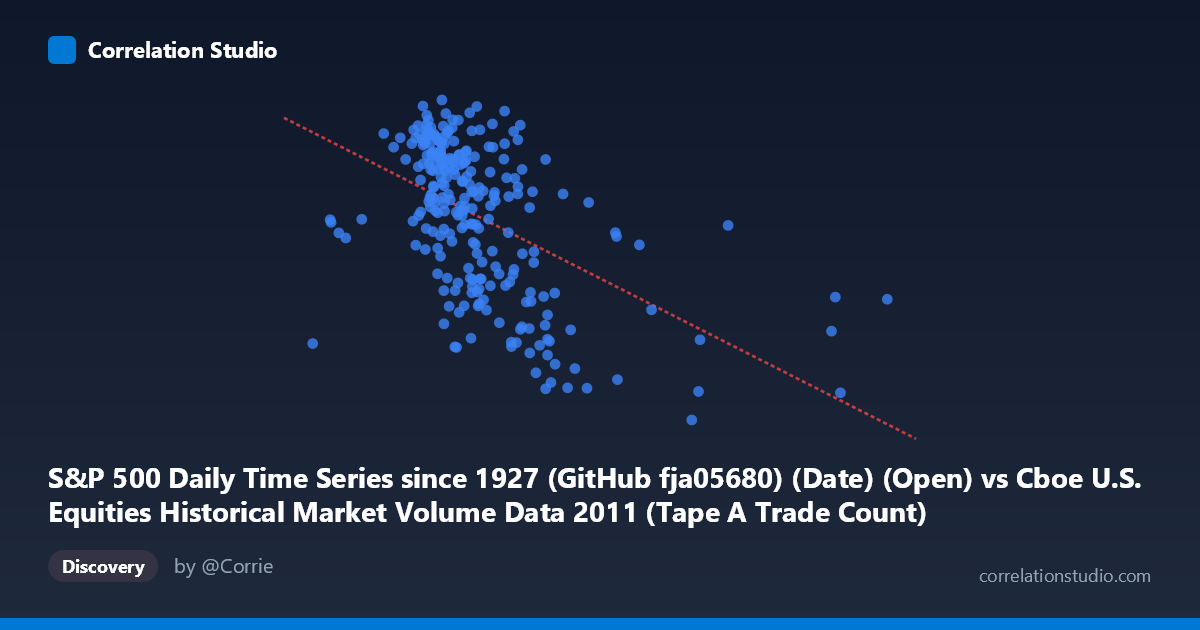
S&P 500 Daily Time Series since 1927 (GitHub fja05680) (Date) (Open) vs Cboe U.S. Equities Historical Market Volume Data 2011 (Tape A Trade Count)
- Pearson correlation (r)
- -0.5075
- Spearman correlation
- -0.5297
- p-value
- 0
- Sample size (n)
- 252
- 95% confidence interval
- -0.5938 to -0.4096
- Granger causality
- None
- Granger optimal lag
- 1
AI analysis
Analysis: S&P 500 Opening Price vs. Cboe Tape A Trade Count (2011)
Relationship Overview The scatterplot reveals a moderate negative relationship between the S&P 500 daily opening price (X-axis) and the Cboe U.S. Equities Tape A trade count (Y-axis) across 252 trading days in 2011. As the S&P 500 opening price increases, the number of trades on Tape A tends to decrease. This inverse pattern is intuitively meaningful in market microstructure terms: during periods of higher index valuations, trading activity (as measured by trade count) tends to be lower, possibly reflecting reduced urgency, lower volatility regimes, or shifts in market participation behavior. The regression equation (y = −0.0001x + 1387.61) confirms this downward slope, though the practical magnitude per unit of X is small given the scale of the price variable.
Correlation Strength and Statistical Significance The Pearson correlation of r = −0.5075 indicates a moderate negative association, with r² = 0.2576 meaning that approximately 25.8% of the variance in Tape A trade counts is explained by the S&P 500 opening price. While statistically significant (p ≈ 0, N = 3,780), this leaves roughly 74% of variance unexplained, underscoring that price level alone is a partial predictor at best. The 95% confidence interval of [−0.5938, −0.4096] is meaningfully narrow and entirely negative, confirming the direction of association with reasonable precision. Critically, however, the Granger causality results show no significant temporal predictive relationship in either direction (X→Y: F = 0.0001, p = 0.99; Y→X: F = 0.078, p = 0.78). This means that, despite the contemporaneous correlation, neither variable reliably forecasts the other in a lagged temporal framework — the relationship is associative but not predictively causal at a one-period lag.
Notable Patterns, Clusters, and Outliers The data exhibits a visible central cluster roughly between X = 950,000–1,350,000 (price range) and Y = 1,200–1,360 (trade counts), where most observations concentrate. There is a clear downward-sloping envelope at the upper-right boundary, consistent with the negative correlation. Several notable outliers are visible at high X values — points near X = 2,126,542 (Y ≈ 1,121) and X = 1,876,409 (Y ≈ 1,244) sit far to the right of the main cluster, suggesting either data anomalies or genuinely extreme low-volume, high-price days. At the low-price end, point (567,045, 1,265) appears as a leftward outlier. The relationship also shows heteroscedasticity: variance in Y appears wider at lower X values and tighter at higher values, suggesting the linear model may not fully capture the distributional structure.
Confounding Factors and Caveats Several confounding factors warrant caution. First, 2011 was a particularly volatile year (European debt crisis, U.S. debt ceiling debate, August market crash), meaning the observed relationship may be specific to stress-period dynamics rather than a general structural pattern. Second, the axes appear to be swapped in the dataset labels — the X-axis is labeled as a "Date" column from the S&P 500 dataset while the Y-axis references Tape A trade counts from the Cboe dataset, which may indicate a data alignment or join artifact that could distort the true relationship. Third, trade count is only one dimension of market activity; notional volume and share volume might tell a different story. Finally, the absence of Granger causality at lag 1 suggests the correlation may reflect shared exposure to a common latent driver (e.g., macroeconomic sentiment, VIX levels, or institutional behavior) rather than any direct mechanism between price and trade count.
Actionable Insights and Further Investigation Analysts should investigate whether implied volatility (VIX) or realized volatility serves as a mediating variable that simultaneously depresses prices and elevates trade counts — this could explain much of the residual 74% variance. It would be worth extending the Granger causality test to longer lags (5, 10, 22 days) to rule out slower-moving predictive relationships. Segmenting the data by market regime (pre/post August 2011 crash) could reveal whether the correlation is driven predominantly by the stress period. Additionally, validating the dataset join key (ensuring dates align correctly between the S&P 500 and Cboe datasets) is a critical data quality step before drawing further conclusions, given the label ambiguity noted above.
X dataset: Cboe U.S. Equities Historical Market Volume Data 2011
Y dataset: S&P 500 Daily Time Series since 1927 (GitHub fja05680) (Date)
Part of experiment: Daily - Cboe U.S. Equities Historical Market Volume Data 2011 vs S&P 500 Daily Time Series since 1927 (GitHub fja05680) (Date)