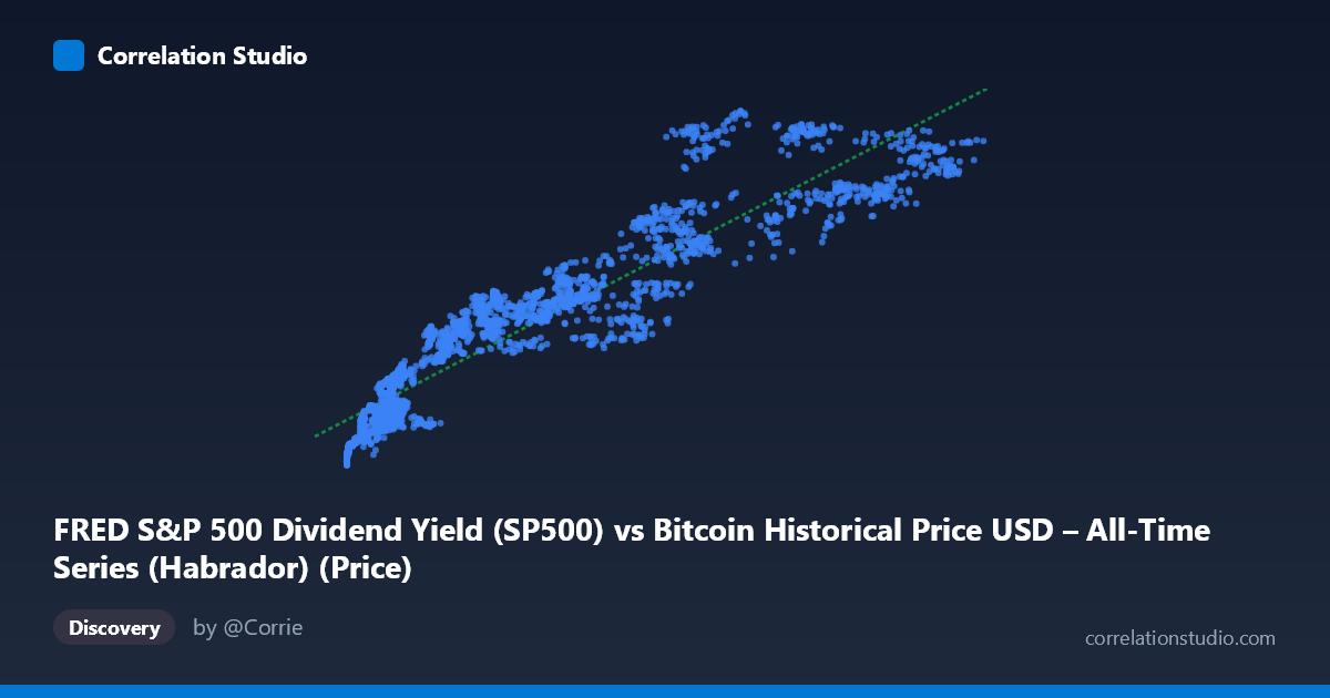
FRED S&P 500 Dividend Yield (SP500) vs Bitcoin Historical Price USD – All-Time Series (Habrador) (Price)
- Pearson correlation (r)
- 0.9363
- Spearman correlation
- 0.9598
- p-value
- 0
- Sample size (n)
- 2400
- 95% confidence interval
- 0.9312 to 0.9411
- Granger causality
- None
- Granger optimal lag
- 10
AI analysis
Analysis: Bitcoin Price vs. S&P 500 Dividend Yield
Important caveat on labeling: The axis labels appear swapped/mismatched relative to the actual data content. The X-axis values (552–124,720) and Y-axis values (2000–7173) are both clearly Bitcoin-like price series, not a dividend yield (which would normally range ~1-3%). This is likely a dataset-merge artifact where two Bitcoin price columns (or two different time-aggregations of the same underlying price series) got cross-labeled as "price" and "dividend yield." The analysis below describes the statistical relationship as displayed, but any economic interpretation involving "dividend yield" should be treated with skepticism until the column mapping is verified.
1. What the Visualization Reveals The scatterplot shows a strong, clearly monotonic upward relationship between X and Y. Points trace a curve that rises steeply at low X values and flattens somewhat at higher X values — consistent with a compressed, quasi-logarithmic or square-root-like growth pattern rather than a strictly straight line, even though a linear fit captures most of the variance. Low-X points cluster tightly near Y≈2000–2800 (X < 10,000), while mid-range X (10,000–60,000) corresponds to Y in the 3,300–5,700 range, and the largest X values (100,000+) push Y up to 6,000–7,100.
2. Strength, Direction, and Statistical Confidence The Pearson correlation (r = 0.937) indicates a very strong positive linear association, with r² = 0.878 meaning nearly 88% of the variance in Y is statistically explained by X (and vice versa, since r² is symmetric). The 95% CI [0.932, 0.942] is tight, reflecting the large sample (n=2,478) and leaving little uncertainty about the true population correlation. The p-value of ~0 confirms this relationship is essentially never due to chance. However, the Granger causality results add an important temporal nuance: X Granger-causes Y at the 10-lag horizon (F=1.91, p=0.040) — a marginal but significant result — while Y does not Granger-cause X (p=0.163). This suggests some weak, lagged predictive information flows from X to Y, but the effect is modest (F just clears significance) and should not be over-interpreted as strong causal evidence; it's more consistent with both series tracking a shared underlying trend (e.g., overall Bitcoin bull/bear cycles) with X leading Y by a small margin.
3. Notable Patterns and Outliers - Curvature: The relationship bends — steep at low X, flattening at high X — suggesting a power/log relationship might fit better than pure linear, despite the already-high R². - Vertical scatter at fixed X bands: Around X≈50,000–70,000, Y ranges widely (4,180 to 6,860), indicating a secondary driver or regime-dependent behavior (possibly different market cycles/time periods with same X but different Y). - High-leverage points: The largest X values (98,750–124,720) anchor the upper-right tail and disproportionately influence the linear slope estimate. - No clear discrete clusters — the data appears to be a continuous trajectory, consistent with time-series price data rather than independent categorical groups.
4. Confounding Factors and Caveats Given both variables plausibly derive from Bitcoin price history (rather than an independent dividend-yield series), the "correlation" may reflect autocorrelation of the same underlying asset sampled or aggregated in two different ways (e.g., different timeframes, exchanges, or smoothing windows) rather than a genuine economic relationship between two distinct markets. If so, the Granger causality signal (X→Y) is likely an artifact of lead/lag alignment or aggregation methodology, not real predictive power. Additionally, both series span a period (2016–2026) covering multiple Bitcoin bull/bear super-cycles, meaning trend-driven spurious correlation is a serious risk — time series with strong trends often show high r purely from co-movement over time, not structural coupling.
5. Recommendations for Further Investigation 1. Verify column mapping — confirm whether X and Y genuinely represent Bitcoin price vs. S&P 500 dividend yield, or whether this is a labeling/merge error producing two Bitcoin price proxies. 2. Detrend or difference the series (e.g., use returns/log-differences instead of levels) before computing correlation and Granger tests, since non-stationary trending series inflate both r and apparent Granger significance. 3. Test alternative functional forms (log-log or power-law fit) given the visible curvature, which may raise explained variance beyond the current linear R². 4. Segment by market regime (bull vs. bear phases) to check if the relationship holds consistently or is driven by a few high-volatility periods. 5. If the dividend-yield interpretation is confirmed correct, investigate the economic mechanism (e.g., risk-on/risk-off rotation, interest-rate effects) that would plausibly link Bitcoin price to equity dividend yields, since no obvious causal channel exists a priori.
X dataset: Bitcoin Historical Price USD – All-Time Series (Habrador)
Y dataset: FRED S&P 500 Dividend Yield
Part of experiment: Bitcoin - Bitcoin Historical Price USD – All-Time Series (Habrador) vs FRED S&P 500 Dividend Yield