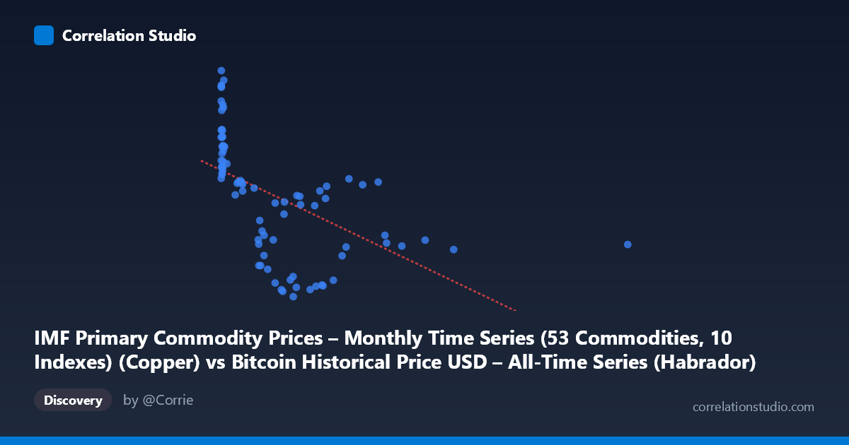
IMF Primary Commodity Prices – Monthly Time Series (53 Commodities, 10 Indexes) (Copper) vs Bitcoin Historical Price USD – All-Time Series (Habrador) (Price)
- Pearson correlation (r)
- -0.5411
- Spearman correlation
- -0.769
- p-value
- 0
- Sample size (n)
- 83
- 95% confidence interval
- -0.6777 to -0.3683
- Granger causality
- None
- Granger optimal lag
- 10
- Time coverage
- 2010-08-01 to 2017-06-01
- Recomputed on refreshed data
- 2026-10-24 (r was -0.5411)
AI analysis
Analysis: Copper Price Index vs. Bitcoin Price (USD)
1. What the Visualization Reveals
The scatterplot shows a moderate negative relationship between the copper commodity price index (X-axis) and Bitcoin's historical USD price (Y-axis). The data reveals a distinctive pattern rather than a simple linear cloud: a dense cluster of points at low X-values (near 0–50) spans an enormous Y-range (roughly 7,300 to 9,880), while as X increases beyond ~200, Y-values compress into a lower band (4,500–7,200) and trend gently downward. This suggests the relationship is driven substantially by a regime shift rather than continuous co-movement.
2. Strength, Direction, and Predictive Value
The Pearson correlation (r = -0.541, r² = 0.293) indicates a moderate negative association, with copper prices explaining only about 29% of the variance in Bitcoin prices — leaving over 70% attributable to other factors. The 95% CI [-0.678, -0.368] is reasonably tight and excludes zero, and the p-value (1.29e-07) confirms this correlation is statistically robust and not due to chance. However, statistical significance should not be conflated with practical strength: with r² well below 0.5, copper price is a weak-to-moderate standalone predictor of Bitcoin price. Critically, the Granger causality tests show no significant predictive direction in either direction (X→Y: p=0.80; Y→X: p=0.30) even at an optimal lag of 10 periods. This means that despite the contemporaneous correlation, neither variable's past values help forecast the other's future values — the relationship is likely coincidental co-trending (e.g., both reacting to broader macroeconomic conditions or simply evolving over the same historical window) rather than a causal or lead-lag dynamic.
3. Notable Patterns and Non-linear Features
The most striking feature is the near-vertical cluster of points at very low copper index values (X < 20) with Y-values spanning almost the entire Bitcoin price range (7,300–9,880). This is likely an artifact of Bitcoin's early price history (2010-2013) coinciding with a period of index scaling or a specific low-value copper index regime, producing high leverage/clustering rather than genuine correlation signal. Beyond this cluster, the relationship flattens into a downward-sloping band for higher X-values. The note that Spearman ρ exceeds Pearson r reinforces that the true relationship is likely monotonic but non-linear — possibly logarithmic or a threshold/step pattern — better fit by a curve (e.g., log(X) or piecewise model) than the straight line y = -1.896x + 7496.81.
4. Confounding Factors and Caveats
This pairing is inherently unusual: it merges a copper commodity index with Bitcoin's price history from an unrelated dataset, joined presumably by date. Both series are non-stationary time series with strong secular trends (Bitcoin's exponential growth trajectory; copper's cyclical macro-driven trend), which is a classic setup for spurious correlation — two trending series can show statistical association without any causal or economic link. Bitcoin's price scale is dominated by its own adoption/speculation cycle (especially the 2013 and 2017 bull runs), which may simply have occurred during a period of relatively low copper prices, mechanically producing negative correlation. Additionally, n=83 sampled points come from a much larger population (N=449 monthly observations), and the low-X cluster may disproportionately influence the linear fit (leverage effect).
5. Suggestions for Further Investigation
Given the lack of Granger causality, this correlation should not be used for predictive trading or forecasting purposes. To properly assess whether any genuine relationship exists: (1) difference or detrend both series (e.g., use returns/log-returns instead of levels) to remove shared trend effects and re-test correlation on stationary data; (2) fit a non-linear model (log or polynomial) as suggested by the Spearman/Pearson gap; (3) investigate the low-X cluster separately, as it may represent a distinct early-Bitcoin regime that should be excluded or modeled separately; and (4) consider a broader macroeconomic control (e.g., USD index, global liquidity/M2) that might be the true common driver behind both series' movements.
X dataset: Bitcoin Historical Price USD – All-Time Series (Habrador)
Y dataset: IMF Primary Commodity Prices – Monthly Time Series (53 Commodities, 10 Indexes)
Part of experiment: Bitcoin - Bitcoin Historical Price USD – All-Time Series (Habrador) vs IMF Primary Commodity Prices – Monthly Time Series (53 Commodities, 10 Indexes)