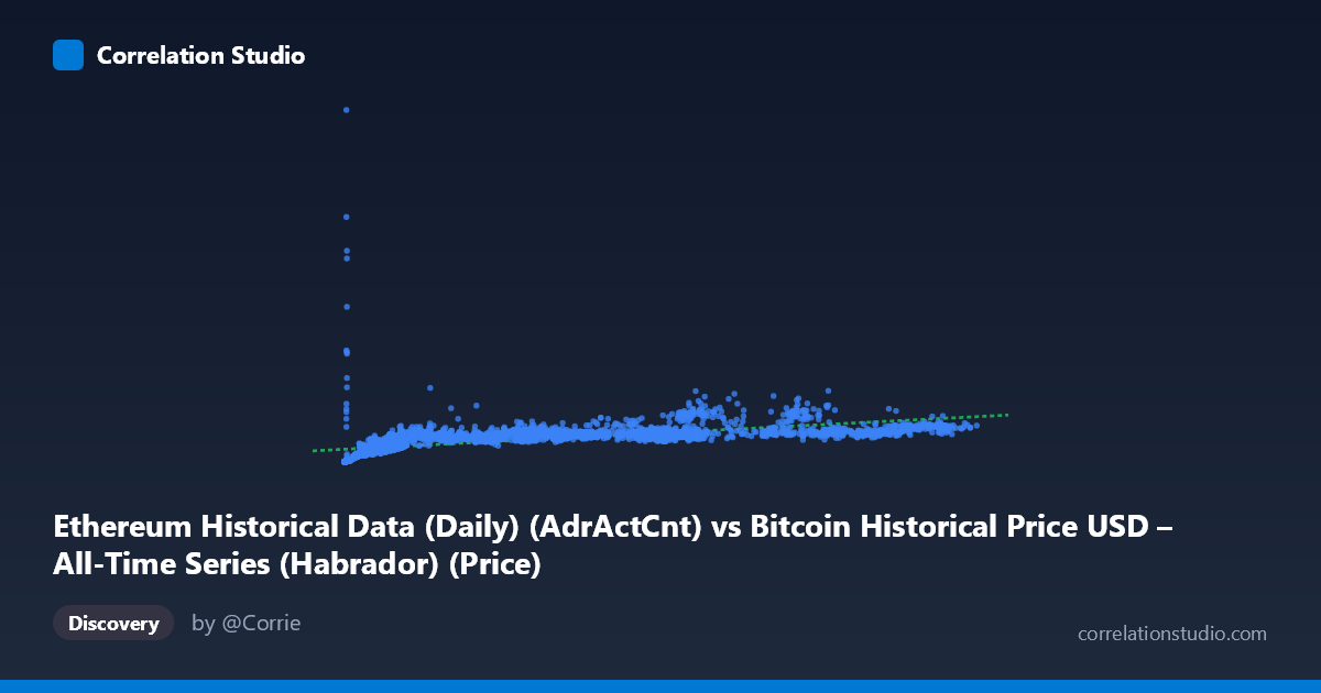
Ethereum Historical Data (Daily) (AdrActCnt) vs Bitcoin Historical Price USD – All-Time Series (Habrador) (Price)
- Pearson correlation (r)
- 0.5775
- Spearman correlation
- 0.8901
- p-value
- 0
- Sample size (n)
- 3926
- 95% confidence interval
- 0.5563 to 0.598
- Granger causality
- None
- Granger optimal lag
- 10
- Time coverage
- 2015-07-30 to 2026-04-28
AI analysis
Analysis: Ethereum Active Address Count vs. Bitcoin Price
1. Overall Relationship
The scatterplot displays a moderate positive relationship between Ethereum's daily active address count (X) and Bitcoin's daily USD price (Y). Despite the mismatched labeling in the metadata (column names appear swapped between the dataset descriptions), the data itself shows a clear pattern: as active address counts rise, Bitcoin price tends to rise as well, though with substantial scatter and evidence of a curved (concave) rather than strictly linear trend. Low-X values cluster tightly at low-Y values (e.g., addresses under 1,000 correspond to prices under $40,000), while higher X values show much wider Y dispersion — a classic sign of heteroscedasticity and non-linear scaling.
2. Strength, Direction, and Statistical Confidence
The Pearson correlation of r = 0.578 indicates a moderate positive linear association, with r² = 0.334 meaning only about 33% of the variance in Bitcoin price is explained by active address count in a linear framework — leaving roughly two-thirds of price movement unexplained by this variable alone. The 95% CI [0.556, 0.598] is tight given the large sample (n=3,926), and the p-value of ~0 confirms this correlation is highly statistically significant and not due to chance. However, statistical significance ≠ practical strength: with r² near 1/3, this is a real but incomplete relationship — useful as one input among many, not a standalone predictor.
Critically, the Granger causality tests show no significant predictive direction in either direction (X→Y: p=0.59; Y→X: p=0.89) at the optimal 10-period lag. This means neither variable reliably "leads" the other in time — the correlation is likely driven by both series responding to a shared underlying factor (overall crypto market cycles, macro liquidity, speculative sentiment) rather than one causing the other. This is an important distinction: correlation here should not be interpreted as one metric forecasting the other.
3. Notable Patterns and Non-linear Features
The data shows a fan-shaped/heteroscedastic pattern: variance in Y increases substantially as X increases. At low X (under ~2,000), Y values are tightly bound below $50,000. At high X (above 70,000), Y ranges widely from ~$460,000 to over $1,280,000 — a nearly 3x spread. This, combined with the note that Spearman ρ exceeds Pearson r, strongly suggests the true relationship is non-linear, likely logarithmic or power-law in nature — consistent with how both blockchain network activity and asset prices tend to grow multiplicatively/exponentially during adoption cycles rather than linearly. A log-log or log-linear transformation would likely produce a much better fit and higher explained variance than the current linear model.
4. Confounding Factors and Caveats
Several caveats apply: (1) Metadata inconsistency — the column labels for X and Y appear mismatched relative to the dataset descriptions (Ethereum address count vs. Bitcoin price data mixed across datasets), so verify field mapping before drawing conclusions. (2) Shared temporal trend: both crypto network usage and crypto prices have grown/cycled together since 2015 due to overall market maturation, making the correlation partly an artifact of co-trending time series rather than a direct mechanical link. (3) Non-stationarity: crypto price and adoption metrics are notoriously non-stationary, which can inflate correlation estimates and invalidates standard Granger causality assumptions unless the series were differenced/detrended first. (4) Bull/bear cycle regimes (2015–2026 span includes multiple boom-bust cycles) could dominate the correlation, with the relationship possibly being much weaker or stronger within specific sub-periods.
5. Actionable Insights
- Re-run correlation on log-transformed variables (log X, log Y) to test the suspected non-linear/power-law relationship, which likely explains more variance. - Test for stationarity (ADF/KPSS tests) and consider differencing or percentage-change transformations before re-running Granger causality, since raw non-stationary series can produce misleading causality results. - Segment by market regime (bull vs. bear cycles) to see if the correlation strengthens or weakens conditionally. - Treat active address count as a supplementary indicator, not a standalone predictive signal, given the lack of Granger causality and moderate r². - Investigate a plausible common driver (e.g., total crypto market cap, macro liquidity/interest rates, or overall investor sentiment indices) that may explain the shared variance between both series more directly.
X dataset: Bitcoin Historical Price USD – All-Time Series (Habrador)
Y dataset: Ethereum Historical Data (Daily)
Part of experiment: Bitcoin - Bitcoin Historical Price USD – All-Time Series (Habrador) vs Ethereum Historical Data (Daily)