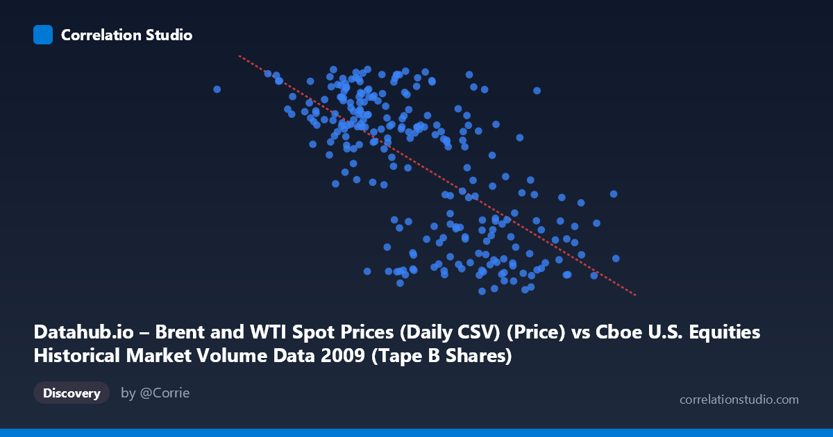
Datahub.io – Brent and WTI Spot Prices (Daily CSV) (Price) vs Cboe U.S. Equities Historical Market Volume Data 2009 (Tape B Shares)
- Pearson correlation (r)
- -0.6659
- Spearman correlation
- -0.6473
- p-value
- 0
- Sample size (n)
- 252
- 95% confidence interval
- -0.7294 to -0.5909
- Granger causality
- None
- Granger optimal lag
- 1
AI analysis
Scatterplot Analysis: Oil Prices vs. Cboe Tape B Share Volume (2009)
Relationship Overview
The scatterplot reveals a moderately strong negative relationship between U.S. equity market volume (Tape B shares, on the X-axis) and Brent/WTI oil spot prices (on the Y-axis) across 252 trading days in 2009. As trading volume increases, oil prices tend to decrease, and vice versa. The linear regression equation (y = -1.92118E-07x + 89.95) quantifies this inverse slope: for every ~5.2 million additional shares traded, oil prices decline by approximately $1 per barrel. Visually, the data occupies a broad diagonal band running from the upper-left (low volume, high oil price) to the lower-right (high volume, low oil price), consistent with this inverse pattern.
Correlation Strength and Statistical Framing
The Pearson correlation of r = -0.666 indicates a moderate-to-strong negative linear association. More precisely, r² = 0.443, meaning that roughly 44.3% of the variance in oil prices is explained by equity trading volume — a meaningful but far from complete explanation, leaving 55.7% of variance attributable to other factors. The 95% confidence interval of [-0.729, -0.591] is relatively tight and does not include zero, and the p-value is effectively zero (p ≈ 0), confirming this association is highly statistically significant across the population of N = 3,232 observations. However, the Granger causality analysis complicates the narrative substantially: neither direction (X→Y nor Y→X) achieves significance (F = 0.087, p = 0.769 and F = 0.789, p = 0.375, respectively). This means that past values of trading volume do not reliably predict future oil prices, and past oil prices do not predict future trading volume at a 1-period lag — suggesting the correlation is contemporaneous and not driven by a clear temporal lead-lag mechanism.
Notable Patterns, Clusters, and Outliers
Several structural features are visible in the data. There appear to be two loosely separated clusters: one concentrated in the lower-right quadrant (high volume ~150–255M shares, low oil prices ~40–55 USD/barrel) and another in the upper-left (lower volume ~65–140M shares, higher oil prices ~65–78 USD/barrel). This bimodal clustering hints at possible regime shifts during 2009 — consistent with the known market context of post-financial crisis recovery, where early-year panic selling drove both high volumes and depressed commodity prices, while later stabilization brought lower volume and recovering oil prices. A few notable outliers are present, including the point at approximately (33.8M shares, 75.15 USD) — an unusually low-volume day with relatively high oil prices — and several high-volume observations around 254M shares with mid-range oil prices (~56 USD), which deviate from the tightest portion of the trend line. The spread of residuals widens at moderate X values, suggesting mild heteroscedasticity.
Confounding Factors and Caveats
Several important caveats apply to this correlation. First, 2009 was an extraordinary year — the global financial crisis bottomed out in Q1, followed by a sharp equity and commodity recovery, meaning both variables were simultaneously driven by the same macro shock (risk-off/risk-on sentiment cycles) rather than directly influencing each other. This is a classic confounding-by-common-cause scenario. Second, Tape B shares represent only a subset of U.S. equity volume (NYSE MKT/AMEX-listed securities), which may not fully represent broader market activity. Third, the absence of Granger causality is a strong caution against any causal interpretation — the correlation likely reflects simultaneous responses to shared economic drivers (e.g., investor risk appetite, macroeconomic news) rather than a mechanistic link. Fourth, daily sampling may obscure intraday dynamics, and the 1-period optimal lag tested may be too short to capture longer feedback cycles.
Actionable Insights and Further Investigation
Despite the non-causal Granger result, the correlation is strong enough to warrant further exploration. Analysts should consider controlling for macroeconomic confounders — such as VIX (volatility index), USD index, or economic surprise indices — to test whether the volume-oil relationship persists after accounting for shared sentiment drivers. It would be valuable to extend the time series beyond 2009 to determine whether this relationship is structurally persistent or idiosyncratic to crisis-recovery dynamics. Testing longer Granger lags (e.g., 5–10 days) could reveal delayed feedback effects not captured at lag-1. Additionally, decomposing the data by calendar quarter would help isolate whether the apparent clustering reflects distinct market regimes during the crisis trough (Q1) versus recovery (Q3–Q4). Finally, a nonlinear or regime-switching model may outperform the linear regression given the visible clustering, and could more accurately characterize the conditional relationship between equity market activity and energy pricing.
X dataset: Cboe U.S. Equities Historical Market Volume Data 2009
Y dataset: Datahub.io – Brent and WTI Spot Prices (Daily CSV)
Part of experiment: Daily - Cboe U.S. Equities Historical Market Volume Data 2009 vs Datahub.io – Brent and WTI Spot Prices (Daily CSV)