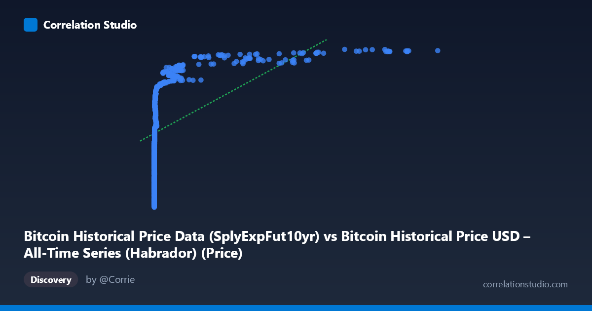
Bitcoin Historical Price Data (SplyExpFut10yr) vs Bitcoin Historical Price USD – All-Time Series (Habrador) (Price)
- Pearson correlation (r)
- 0.5386
- Spearman correlation
- 0.9723
- p-value
- 0
- Sample size (n)
- 721
- 95% confidence interval
- 0.4847 to 0.5885
- Granger causality
- None
- Granger optimal lag
- 10
AI analysis
Analysis: Bitcoin Supply-Adjusted Future Metric vs. Historical Price
1. Relationship Overview
The scatterplot compares an X-axis variable derived from Bitcoin's supply-expansion/futures-adjusted metric (SplyExpFut10yr) against actual historical USD price. The data reveals a clear monotonic but non-linear relationship: as X increases from near-zero values (0.05–15 range, dominating the low end) through mid-range values (hundreds to thousands) to large values (tens of thousands to 117,410), Y climbs from ~$18M to ~$20.8M in a compressed, curved fashion. The sample points show extreme right-skew in X (mean 6,997 vs. median likely far lower, given stdev of 18,619), while Y is comparatively tight and linearly progressing — classic signature of a logarithmic or power-law relationship rather than a straight line.
2. Strength, Direction, and Statistical Confidence
The Pearson correlation (r = 0.539) indicates a moderate positive relationship, with R² = 0.290 meaning only 29% of the variance in Y is explained by a linear fit with X — leaving 71% unexplained by this simple model. The 95% CI [0.485, 0.589] is reasonably tight given n=721, and p≈0 confirms this correlation is highly unlikely due to chance. However, the note that Spearman ρ exceeds Pearson r is critical: it signals the rank-order relationship is stronger than the linear one, reinforcing that a log/power transformation of X would likely explain substantially more variance. The Granger causality results are equally important: neither direction shows significant predictive causality (X→Y p=0.76, Y→X p=0.166), meaning despite the contemporaneous correlation, past values of one series do not reliably forecast future values of the other in this framework — this is likely because both series are largely deterministic/monotonic transformations of the same underlying time index rather than independently evolving causal systems.
3. Patterns, Clusters, and Outliers
The sample points show a highly compressed cluster near X≈0–20 (representing early Bitcoin history, prices $18M–19.2M in this scaled representation) contrasted with a sparse tail of large X values (37,000–117,000) corresponding to the highest Y values (~20.6–20.8M). This bimodal density — many small-X points, few large-X points — combined with smoothly increasing Y suggests logarithmic compression: equal jumps in ln(X) correspond to roughly equal jumps in Y. There's no evidence of reversals, plateaus, or bimodal clusters in Y itself; the growth pattern appears saturating (diminishing returns) at high X.
4. Confounding Factors and Caveats
The most significant caveat: both axes are almost certainly derived from Bitcoin price and time, since X is a "supply-expansion/futures" metric and Y is literal historical price — they are not independent phenomena but mathematically/temporally linked constructs. This makes classic causal or correlational interpretation inappropriate; the relationship reflects shared temporal trend (both increase as Bitcoin matures and time progresses) rather than one variable driving the other. This also explains the null Granger causality — with both series essentially monotonic functions of calendar time, lagged cross-prediction adds no information beyond each series' own trend. Additionally, the extreme skew in X (a few huge values vs. many near-zero) means the linear correlation coefficient is heavily influenced by leverage points at the high end.
5. Recommendations
1. Re-fit with log(X): Given the Spearman/Pearson divergence and visible saturation curve, test y = a·ln(x) + b or a power-law model — this will likely raise R² substantially above 0.29. 2. Detrend for time: Since both series likely correlate with elapsed time, compute partial correlation controlling for date/period to isolate any genuine relationship beyond shared trend. 3. Treat Granger results as expected null: Given probable definitional overlap between X and Y, causality testing may be conceptually moot — clarify the exact construction of the "SplyExpFut10yr" metric to confirm whether it's already a price-derived quantity. 4. Segment analysis: Compare early era (X<1000) vs. modern era (X10,000) separately, as the relationship's slope/shape may differ across Bitcoin's early speculative years vs. mature-market years.
X dataset: Bitcoin Historical Price USD – All-Time Series (Habrador)
Y dataset: Bitcoin Historical Price Data
Part of experiment: Bitcoin - Bitcoin Historical Price USD – All-Time Series (Habrador) vs Bitcoin Historical Price Data