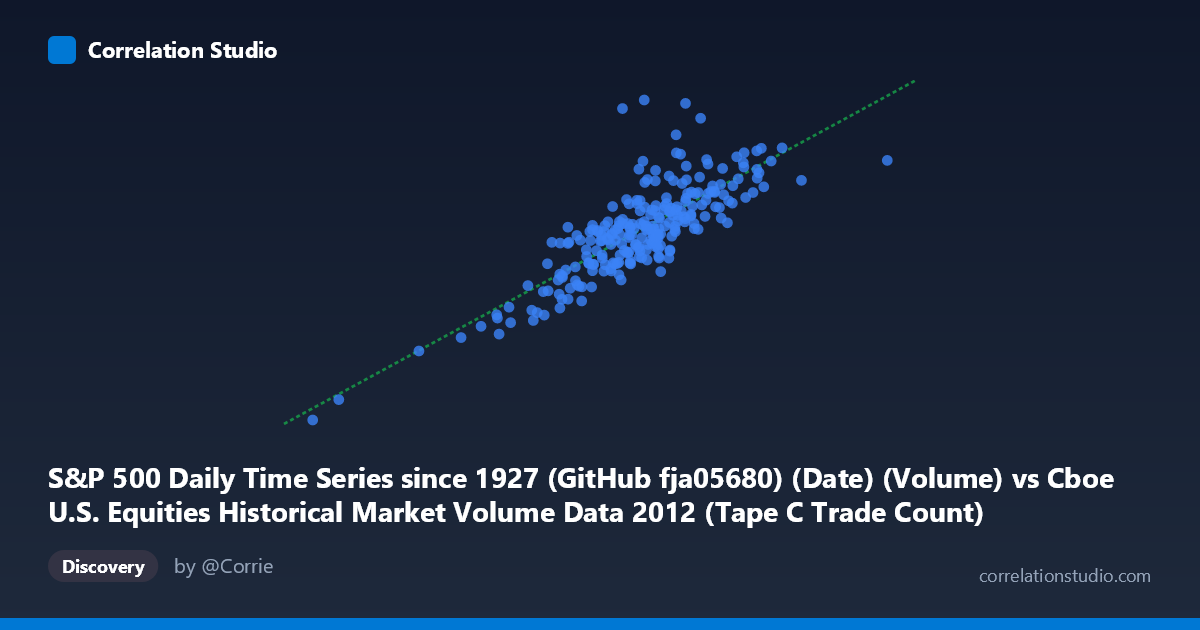
S&P 500 Daily Time Series since 1927 (GitHub fja05680) (Date) (Volume) vs Cboe U.S. Equities Historical Market Volume Data 2012 (Tape C Trade Count)
- Pearson correlation (r)
- 0.8143
- Spearman correlation
- 0.7893
- p-value
- 0
- Sample size (n)
- 250
- 95% confidence interval
- 0.7678 to 0.8522
- Granger causality
- X → Y
- Granger optimal lag
- 10
AI analysis
Scatterplot Analysis: S&P 500 Volume vs. Cboe Tape C Trade Count (2012)
Relationship Overview The scatterplot reveals a clear, positive linear relationship between S&P 500 daily trading volume (X-axis) and Cboe U.S. Equities Tape C trade count (Y-axis) across 250 trading days in 2012. As daily volume increases, the number of discrete trades on Tape C rises correspondingly, which is intuitively sensible — higher volume days tend to involve more individual transactions rather than simply larger block trades. The linear regression equation (y = 7,565.97x + 9.25×10⁷) suggests that each unit increase in volume is associated with approximately 7,566 additional Tape C trades, with a substantial baseline intercept reflecting the minimum transaction activity present even on lower-volume days.
Correlation Strength and Statistical Significance The Pearson correlation of r = 0.8143 indicates a strong positive association, and the coefficient of determination r² = 0.6630 means that roughly 66.3% of the variance in Tape C trade counts is statistically explained by S&P 500 volume — a meaningful but incomplete explanatory relationship, leaving about one-third of variance attributable to other factors. The 95% confidence interval of [0.7678, 0.8522] is notably narrow given the sample size of n = 250 drawn from N = 3,750, and the p-value of effectively zero confirms this correlation is not a chance artifact. Critically, Granger causality runs unidirectionally from X→Y (F = 2.2374, p = 0.0168) at an optimal lag of 10 trading periods, meaning S&P 500 volume has statistically significant temporal predictive power over Tape C trade counts approximately two calendar weeks later. The reverse direction (Y→X) fails to reach significance (p = 0.1825), reinforcing that broader market volume dynamics lead exchange-specific trade counts rather than the other way around.
Notable Patterns, Clusters, and Outliers The data cloud shows reasonably tight clustering in the central range (X: ~420,000–540,000; Y: ~3.2B–4.2B), consistent with typical 2012 trading conditions. However, several notable outliers are visible. One point near (471,858; 5,271,490,000) sits dramatically above the regression line, representing an anomalous spike in Tape C trade counts disproportionate to its volume level — likely corresponding to a specific market event such as an options expiration, index rebalancing, or flash-volatility episode. Similarly, the lower-left cluster around (338,540–380,000; 2,500,000,000–2,600,000,000) suggests episodic low-activity days, potentially surrounding holidays or summer lulls. The spread of residuals appears to widen slightly at higher volume levels, hinting at mild heteroscedasticity — high-volume days produce more variable trade counts, consistent with the diversity of market conditions that can drive surges.
Confounding Factors and Interpretive Caveats Several important caveats temper interpretation. First, both variables are driven by common macro factors — market volatility (VIX spikes), major economic announcements (FOMC decisions, NFP releases), and end-of-quarter rebalancing — meaning the correlation partially reflects shared external forcing rather than a direct causal mechanism. Second, the 10-period Granger lag (roughly two weeks) is suggestive but Granger causality does not establish structural causation; it may reflect persistent volatility regimes rather than a true volume→trade-count transmission mechanism. Third, Tape C specifically covers NYSE Arca-listed securities, so its trade count reflects a subset of total market activity; compositional shifts in which securities dominate on any given day could distort the relationship. Finally, the 2012 time window captures a specific post-crisis recovery regime, limiting generalizability to other market environments.
Actionable Insights and Further Investigation Practitioners monitoring Tape C market microstructure could use lagged S&P 500 volume as a leading indicator for anticipated trade-count load, valuable for exchange capacity planning and algorithmic execution scheduling roughly two weeks forward. To deepen understanding, analysts should: (1) decompose residuals to identify which specific dates produce the largest deviations (particularly the extreme upper outlier), potentially linking them to known market events; (2) test non-linear specifications (e.g., log-log regression) given the possible heteroscedasticity; (3) extend the time series across multiple years to assess whether the r² and Granger lag remain stable across different volatility regimes; and (4) include volatility controls (e.g., realized VIX levels) as covariates to isolate the volume→trade-count relationship from shared volatility confounding. The 10-period predictive lag in particular warrants replication on out-of-sample data before being operationalized in any trading or risk management framework.
X dataset: Cboe U.S. Equities Historical Market Volume Data 2012
Y dataset: S&P 500 Daily Time Series since 1927 (GitHub fja05680) (Date)
Part of experiment: Daily - Cboe U.S. Equities Historical Market Volume Data 2012 vs S&P 500 Daily Time Series since 1927 (GitHub fja05680) (Date)