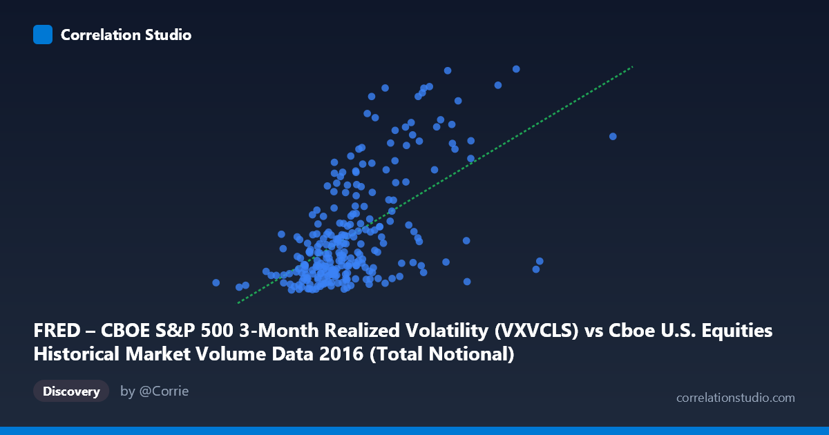
FRED – CBOE S&P 500 3-Month Realized Volatility (VXVCLS) vs Cboe U.S. Equities Historical Market Volume Data 2016 (Total Notional)
- Pearson correlation (r)
- 0.5751
- Spearman correlation
- 0.5478
- p-value
- 0
- Sample size (n)
- 252
- 95% confidence interval
- 0.486 to 0.6523
- Granger causality
- None
- Granger optimal lag
- 1
AI analysis
Analysis: CBOE S&P 500 3-Month Realized Volatility vs. U.S. Equities Total Notional Volume (2016)
1. Overall Relationship The scatterplot reveals a moderate positive relationship between CBOE S&P 500 3-month realized volatility (VXVCLS) and total notional trading volume in U.S. equities markets during 2016. As realized volatility increases, notional volume tends to rise as well — a directionally intuitive finding, since heightened uncertainty in equity markets typically drives greater trading activity. The linear regression equation (y = 4.10×10⁻¹⁰x + 10.46) confirms this upward slope, though the scatter around the regression line is substantial, indicating that volatility alone is far from a complete explanation of volume behavior.
2. Correlation Strength and Statistical Framing The correlation of r = 0.5751 is statistically significant (p ≈ 0, N = 3,622), but the more telling metric is r² = 0.3307 — meaning realized volatility explains only about 33% of the variance in total notional volume, leaving roughly two-thirds attributable to other factors. The 95% confidence interval for r [0.486, 0.652] is reasonably tight and does not approach zero, giving confidence in the direction of the relationship, but it spans a wide enough range to reflect meaningful uncertainty about the precise magnitude. Critically, Granger causality tests find no significant predictive direction in either direction (X→Y: F = 0.016, p = 0.899; Y→X: F = 0.674, p = 0.413). This means that past values of volatility do not reliably predict future volume, and vice versa — the two variables move together contemporaneously rather than one leading the other in time. This is an important caveat: the correlation is real, but it does not support a simple predictive or causal trading signal.
3. Notable Patterns, Clusters, and Outliers The sample points reveal at least two visually distinct clusters. The majority of observations are concentrated in the lower-left region — volatility roughly between 12–22 billion (notional X range) and realized vol between 15–20 — suggesting that during most of 2016, markets were in a relatively calm, range-bound regime. However, a clear upper-right cluster of high-leverage outliers is visible (e.g., points near (25×10⁹, 26.7) and (20.3×10⁹, 25.25)), likely corresponding to discrete market stress events such as the Brexit vote in late June 2016 or the U.S. presidential election in November. These high-volatility, high-volume episodes exert disproportionate influence on the regression slope and the overall correlation coefficient, which may inflate r beyond what holds in calmer regimes.
4. Confounding Factors and Caveats Several confounding dynamics deserve attention. First, both variables are likely driven by common external shocks (geopolitical events, macro announcements, Fed policy decisions in 2016) rather than one causing the other — consistent with the failed Granger tests. Second, the VXVCLS measures 3-month realized volatility, introducing a temporal smoothing effect that may obscure day-to-day dynamics; a shorter-horizon volatility measure might produce a different correlation structure. Third, notional volume is sensitive to price levels — if equity prices rise during stress, notional volume could inflate even if share-count volume is unchanged. Fourth, market structure effects in 2016 (e.g., shifts in electronic trading, maker-taker fee changes) could independently drive volume fluctuations unrelated to volatility. Finally, the dataset covers only a single calendar year, limiting generalizability across different volatility regimes.
5. Actionable Insights and Further Investigation Practitioners should avoid using this relationship as a standalone predictive tool given the absence of Granger causality and the 67% unexplained variance. However, several follow-up analyses are warranted. Regime-segmented analysis — separating calm versus stress periods (e.g., pre- and post-Brexit) — would test whether the correlation is driven primarily by a handful of event days. Replacing VXVCLS with a shorter-horizon measure (e.g., VIX or 1-month realized vol) could sharpen temporal alignment with daily volume. A multivariate model incorporating variables such as market returns, bid-ask spreads, and macro release calendars would likely explain substantially more variance. Finally, examining whether this correlation structure holds across multiple years (2014–2023) would clarify whether 2016 is representative or anomalous, particularly given the unusual political events concentrated in that year.
X dataset: Cboe U.S. Equities Historical Market Volume Data 2016
Y dataset: FRED – CBOE S&P 500 3-Month Realized Volatility
Part of experiment: Daily - Cboe U.S. Equities Historical Market Volume Data 2016 vs FRED – CBOE S&P 500 3-Month Realized Volatility