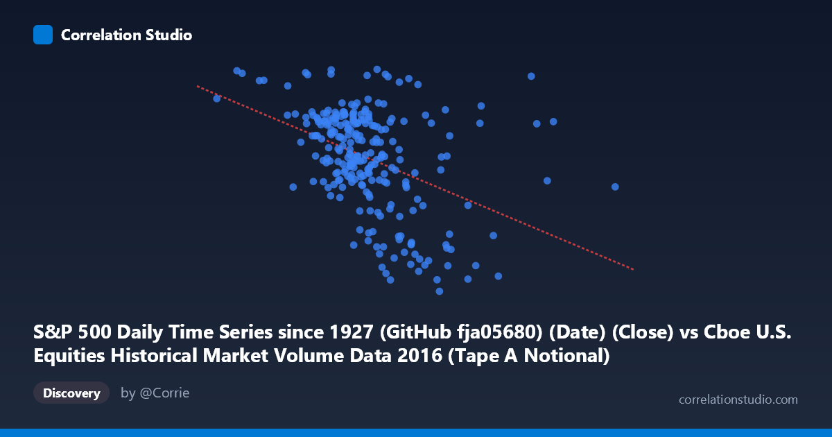
S&P 500 Daily Time Series since 1927 (GitHub fja05680) (Date) (Close) vs Cboe U.S. Equities Historical Market Volume Data 2016 (Tape A Notional)

Pearson correlation (r): -0.4172
Spearman correlation: -0.428
p-value: 0
Sample size (n): 252
95% confidence interval: -0.5143 to -0.3096
Granger causality: None
Granger optimal lag: 4

AI analysis

Scatterplot Analysis: S&P 500 Close Price vs. Tape A Notional Volume (2016)

Relationship Overview The scatterplot reveals a moderate negative relationship between the S&P 500 closing price (X-axis, representing date encoded as a Unix-style timestamp) and Cboe Tape A notional trading volume (Y-axis). As the index price level increased throughout 2016, notional volume on Tape A tended to decline, though with considerable scatter around this trend. The linear regression equation (y = -2.387E-08x + 2309.17) confirms this downward slope, suggesting that higher price levels — which correspond to later dates in 2016 — were associated with somewhat lower aggregate notional volume activity. This likely reflects the well-documented tendency for equity market volatility and volume to compress during calm, steadily rising markets.

Correlation Strength and Statistical Significance The Pearson correlation of r = -0.417 indicates a moderate negative association, but the variance explained is modest: R² = 0.174, meaning only about 17.4% of the variance in Tape A notional volume is explained by the S&P 500 price level. The remaining ~82.6% of variability is driven by other factors entirely. The 95% confidence interval for r spans [-0.514, -0.310], which is meaningfully negative throughout and does not cross zero, reinforcing that the negative direction is reliable. The p-value of 4.93E-12 is highly significant given n = 252 paired observations, making it extremely unlikely this correlation arose by chance. However, statistical significance here is partly a function of sample size and should not be conflated with practical or economic importance. Critically, the Granger causality tests show no significant predictive direction in either direction (X→Y: F = 0.41, p = 0.80; Y→X: F = 1.08, p = 0.37), meaning that knowing the S&P 500 price level does not help predict future notional volume, and vice versa — the correlation is associative, not temporally predictive.

Notable Patterns, Clusters, and Outliers Several structural features stand out in the data. There is a visible cluster of points in the mid-range (X approximately 7.5B–9.5B, Y approximately 2050–2200), representing the bulk of trading days where volume was relatively stable. A distinct low-volume cluster appears at higher X values (roughly 10B–11B), corresponding to later-year dates when the S&P 500 was elevated — these points pull the regression slope downward and likely represent quieter summer or pre-election trading periods. Conversely, a few high-notional-volume outliers appear at lower X values and elevated Y values (e.g., ~6.78B, 2265 and ~9.58B, 2262), which may correspond to specific high-volatility events or option expiration dates. One notable low-volume outlier cluster around X = 10.5B–10.8B with Y near 1870–1895 represents exceptionally thin volume days at elevated price levels. The overall spread in Y (~443 points range) is substantial relative to the trend line's explanatory power, visually confirming the low R².

Confounding Factors and Caveats A critical interpretive caveat is that the X-axis is fundamentally a date variable encoded numerically — so this correlation is largely capturing a time trend rather than a direct price-volume relationship. Both series are evolving through time simultaneously, meaning any shared temporal drift (e.g., seasonal volume patterns, the 2016 election cycle, post-Brexit volatility in H1 vs. calm in H2) could manufacture or inflate the observed correlation. Additionally, notional value conflates price and share volume — as the S&P 500 rises, the same number of shares traded generates higher notional values, which would create an upward bias that partially offsets the observed negative relationship. The negative correlation persisting despite this suggests actual share volume declined meaningfully later in the year. Selection bias in the 252-sample drawn from a population of 3,622 records also warrants caution, and the dataset covers only a single calendar year, limiting generalizability.

Actionable Insights and Further Investigation Practitioners should decompose the X variable into its temporal and price components separately — regressing notional volume against both calendar date and S&P 500 price level independently to isolate whether it is the timing or price level driving volume changes. A rolling volatility measure (e.g., VIX) should be incorporated as a covariate, since volatility is a well-established driver of trading volume and likely explains much of the residual 82.6% variance. Investigating specific outlier dates (particularly the high-volume points) against known market events (Brexit aftermath, U.S. election day, FOMC announcements) would clarify whether episodic shocks dominate the distribution. Given the failed Granger causality tests, no trading strategy should be built on using price levels to predict future volume in this dataset. Extending the analysis across multiple years would test whether the 2016 pattern is idiosyncratic or structurally persistent.

X dataset: Cboe U.S. Equities Historical Market Volume Data 2016

Y dataset: S&P 500 Daily Time Series since 1927 (GitHub fja05680) (Date)

Part of experiment: Daily - Cboe U.S. Equities Historical Market Volume Data 2016 vs S&P 500 Daily Time Series since 1927 (GitHub fja05680) (Date)