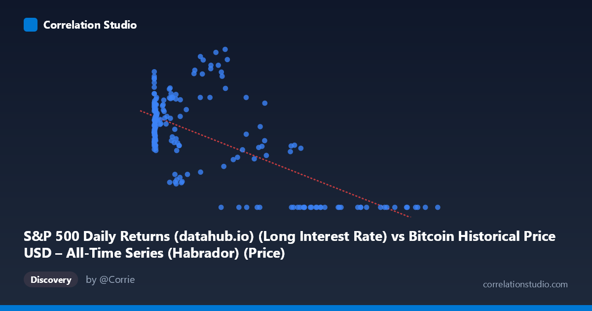
S&P 500 Daily Returns (datahub.io) (Long Interest Rate) vs Bitcoin Historical Price USD – All-Time Series (Habrador) (Price)
- Pearson correlation (r)
- -0.6767
- Spearman correlation
- -0.5167
- p-value
- 0
- Sample size (n)
- 194
- 95% confidence interval
- -0.7464 to -0.5923
- Granger causality
- None
- Granger optimal lag
- 1
- Time coverage
- 2010-08-01 to 2026-09-01
- Recomputed on refreshed data
- 2026-10-24 (r was -0.6533)
AI analysis
Analysis of Bitcoin Price vs. S&P 500-Related Metric
Note on axis labeling: The column labels appear swapped in the metadata (X is labeled as an S&P 500 metric but contains Bitcoin-scale values like 118,670; Y is labeled as Bitcoin price but ranges 0–4.17, consistent with a return or ratio metric). This analysis treats X as the Bitcoin-scale variable (likely price in USD) and Y as a bounded metric (likely a normalized return, ratio, or rate).
1. What the Visualization Reveals
The scatterplot shows a clear negative, non-linear relationship. At low-to-moderate X values (roughly 0–20,000), Y clusters tightly between 1.6 and 4.2, showing high variability but no strong downward trend within that band. However, once X exceeds ~35,000–40,000, Y collapses toward zero almost deterministically — nearly every point above X≈57,000 has Y=0.00. This creates a distinctive "L-shaped" or threshold pattern rather than a uniform linear decay.
2. Strength, Direction, and Statistical Confidence
The Pearson correlation of r = -0.6533 indicates a moderately strong negative relationship, with r² = 0.4268 meaning the linear model explains only 42.7% of the variance in Y — the majority (57%) remains unexplained by X alone, consistent with the non-linear threshold behavior noted above. The 95% CI [-0.7281, -0.5630] is reasonably tight and excludes zero, and the p-value ≈ 0 confirms this correlation is highly unlikely to be due to chance in this sample. However, correlation strength here is partly an artifact of the extreme-value clustering at high X (many zeros) rather than a smooth linear decay — R² would likely improve substantially with a logistic, exponential, or piecewise model.
The Granger causality results are notable: Y Granger-causes X (F=4.8712, p=0.0285) while X does not Granger-cause Y (p=0.365). This suggests that past values of Y have predictive power for future X, not the reverse — an important and possibly counterintuitive finding if X is truly Bitcoin price, since one might expect price to drive returns rather than the other way around.
3. Notable Patterns and Outliers
- Threshold/saturation effect: Y≈0 is essentially a hard floor for X 57,000, suggesting a regime change (e.g., a rate or return metric that mechanically approaches zero as Bitcoin price rises past a certain historical era — possibly reflecting a maturing/declining volatility or yield metric over time). - High-variance low-X cluster: For X < 1,000, Y ranges from 1.6 to 3.6, showing this region carries little predictive signal from X alone — other factors dominate. - Sparse mid-range: Few points populate X between 45,000–56,000, creating a gap that makes the "cliff" to zero look sharper than it may be in reality.
4. Confounding Factors and Caveats
Given the mismatched axis labels, the biggest caveat is metadata/column confusion — it's unclear whether this is truly Bitcoin price vs. a rate, or some other pairing. Time is a critical hidden confounder: Bitcoin's price has grown roughly monotonically with time, and if Y is a rate/yield that has also trended down over the 2010–2026 window (e.g., interest rates, or a declining volatility ratio), the correlation may be substantially driven by shared time trends rather than direct causal interaction. This spurious-trend risk is common in long-run financial time series and should be tested via detrending or first-differencing.
5. Suggestions for Further Investigation
1. Verify column mapping — confirm which variable is genuinely on which axis before drawing substantive conclusions. 2. Test for spurious correlation via detrending: run the correlation on log-differenced or first-differenced series to control for shared time trends. 3. Fit non-linear models (logistic, piecewise, or spline) given the clear threshold behavior, which should improve explanatory power substantially over the linear R²=0.43. 4. Investigate the Granger direction further — given Y→X significance, examine what economic/behavioral mechanism could make Y (e.g., a rate) a leading indicator of X (e.g., Bitcoin price), which would be a genuinely interesting finding worth deeper lag structure analysis (test lags beyond 1 period).
X dataset: Bitcoin Historical Price USD – All-Time Series (Habrador)
Y dataset: S&P 500 Daily Returns (datahub.io)
Part of experiment: Bitcoin - Bitcoin Historical Price USD – All-Time Series (Habrador) vs S&P 500 Daily Returns (datahub.io)