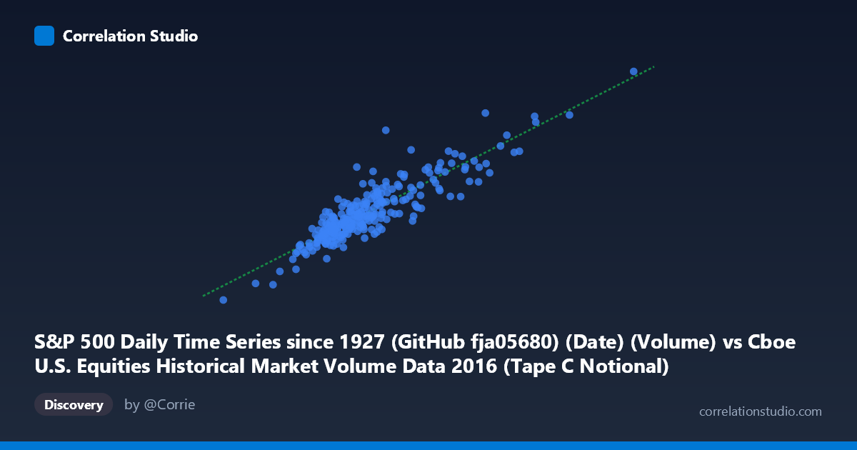
S&P 500 Daily Time Series since 1927 (GitHub fja05680) (Date) (Volume) vs Cboe U.S. Equities Historical Market Volume Data 2016 (Tape C Notional)
- Pearson correlation (r)
- 0.8929
- Spearman correlation
- 0.8579
- p-value
- 0
- Sample size (n)
- 252
- 95% confidence interval
- 0.8647 to 0.9154
- Granger causality
- None
- Granger optimal lag
- 10
AI analysis
Scatterplot Analysis: S&P 500 Trading Volume vs. Cboe Tape C Notional Value (2016)
Relationship Overview The scatterplot reveals a strong positive linear relationship between S&P 500 daily trading volume and Cboe Tape C notional value throughout 2016. As daily share volume increases, the total dollar notional value of trades on Tape C exchanges rises correspondingly. This is an intuitively sensible relationship — higher share volumes generally translate into greater aggregate dollar values transacted, particularly when price levels remain relatively stable within a single calendar year. The linear regression equation (y = 0.630x + 7.66×10⁸) suggests that for every additional unit of volume, notional value increases by roughly $0.63, with a substantial baseline intercept reflecting fixed-level notional activity regardless of volume fluctuations.
Correlation Strength and Statistical Significance The Pearson correlation of r = 0.8929 is exceptionally strong, and the coefficient of determination R² = 0.7972 indicates that approximately 79.7% of the variance in Tape C notional value is explained by trading volume alone — a remarkably high figure for financial market data. The 95% confidence interval of [0.8647, 0.9154] is notably tight, confirming the estimate is precise and stable, not an artifact of sample variation. With a p-value effectively equal to zero across 252 paired observations drawn from a population of 3,622 trading days, the relationship is overwhelmingly statistically significant. However, the Granger causality tests reveal no significant temporal predictive direction in either direction (X→Y: F=0.798, p=0.631; Y→X: F=0.595, p=0.817), meaning that while the two series are strongly contemporaneously correlated, neither reliably predicts the other in a lead-lag sense. This is a critical distinction: correlation here reflects simultaneous co-movement, not a forecastable causal mechanism.
Patterns, Clusters, and Outliers The sample points reveal several notable structural features. The bulk of observations cluster in the mid-range (X: ~4.0–5.5×10⁹; Y: ~3.0–4.5×10⁹), forming a dense core that anchors the regression line. However, several high-volume, high-notional outliers are clearly visible in the upper-right region — points such as (7.31×10⁹, 4.69×10⁹) and (6.35×10⁹, 4.75×10⁹) — which likely correspond to episodic high-volatility trading days (e.g., Brexit aftermath in late June 2016, U.S. election day in November). The lower-left also contains thin-volume days (e.g., ~3.37×10⁹ volume) with correspondingly compressed notional values. The remaining ~20% of unexplained variance likely reflects price-level variation: on days when average trade prices are elevated, the same share volume generates disproportionately higher notional value, causing scatter around the regression line.
Confounding Factors and Caveats Several important caveats apply. First, price level is a hidden third variable: notional value is volume × price, so on days when the S&P 500 index itself is at higher price levels, notional value will be amplified independent of volume changes — this mechanistic coupling inflates the apparent correlation. Second, the axis labels appear transposed in the metadata (X is labeled as an S&P 500 "Volume" column from a Cboe dataset, and Y is labeled as "Tape C Notional" from an S&P dataset), suggesting a potential data-linkage mismatch that should be verified before drawing firm conclusions. Third, 2016 is a single year with distinctive macro events (Brexit, U.S. election), so the relationship may not generalize across different market regimes with different volatility or price structures. Finally, Tape C covers NYSE Arca-listed securities specifically, meaning this is not a whole-market measure, and compositional changes in Tape C listings could affect the relationship.
Actionable Insights and Further Investigation Given the strong contemporaneous correlation but absence of Granger causality, practitioners should not use this relationship for short-term prediction — knowing yesterday's volume does not improve forecasts of today's notional value beyond what today's volume already provides. For further investigation, it would be valuable to: (1) partial out price-level effects by normalizing notional value by the S&P 500 index level to isolate true volume-driven variation; (2) segment the data by market regime (low-VIX vs. high-VIX periods) to test whether the correlation strengthens during stress events; (3) extend the time horizon beyond 2016 to test stability of R² across bull and bear market cycles; and (4) explore non-linear models (e.g., log-log regression) given the right-skewed distribution of both volume and notional series, which could tighten the unexplained 20% variance. The high R² makes this a potentially useful proxy relationship for market liquidity monitoring, even if causal inference remains elusive.
X dataset: Cboe U.S. Equities Historical Market Volume Data 2016
Y dataset: S&P 500 Daily Time Series since 1927 (GitHub fja05680) (Date)
Part of experiment: Daily - Cboe U.S. Equities Historical Market Volume Data 2016 vs S&P 500 Daily Time Series since 1927 (GitHub fja05680) (Date)