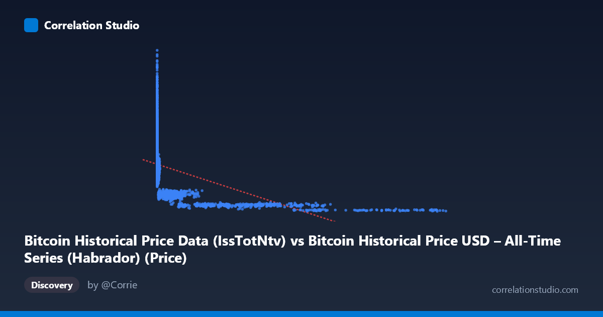
Bitcoin Historical Price Data (IssTotNtv) vs Bitcoin Historical Price USD – All-Time Series (Habrador) (Price)
- Pearson correlation (r)
- -0.4764
- Spearman correlation
- -0.9039
- p-value
- 0
- Sample size (n)
- 3327
- 95% confidence interval
- -0.5022 to -0.4497
- Granger causality
- None
- Granger optimal lag
- 10
- Time coverage
- 2010-07-18 to 2026-04-16
AI analysis
Analysis: Bitcoin Historical Price Data Relationship
1. What the Visualization Reveals
This scatterplot compares two columns that both purport to represent Bitcoin's historical USD price, but sourced from different datasets ("IssTotNtv" field vs. a separate "Price" column). The relationship shown is not a simple linear price-to-price correlation — instead, it reveals a curved, inverse-looking pattern where small X-values correspond to a wide range of Y-values (350–9,800+), while large X-values (tens of thousands) compress into a narrow, low Y-band (800–2,225). This asymmetric funnel shape is a strong signal that X and Y are not measuring the same underlying quantity in the same units or time alignment — otherwise a roughly 1:1 diagonal relationship would be expected for two "price" series.
2. Strength, Direction, and Statistical Uncertainty
The Pearson correlation is r = -0.476 (moderate negative), with r² = 0.227, meaning only about 22.7% of the variance in Y is explained by a linear relationship with X. The 95% CI [-0.502, -0.450] is tight and excludes zero, and the p-value is effectively 0, so despite the modest effect size, the negative association is statistically robust and not due to chance given the large sample (n=3,327). However, statistical significance here reflects sample size more than practical strength — nearly 78% of Y's variance is left unexplained by X alone. Critically, the Granger causality tests show no significant predictive direction (X→Y: p=0.328; Y→X: p=0.827), indicating that neither series temporally leads the other in a way that would support forecasting one from the other's past values. This strongly suggests the correlation is not causal or dynamically linked, but likely an artifact of how the two "price" fields were constructed or scaled.
3. Notable Patterns and Non-linear Features
The sample data shows a clear non-linear, logarithmic-like decay: Y stays elevated (5,000–9,800) while X is very small (<20), then Y steadily declines as X grows into the hundreds and thousands, flattening near 800–2,225 once X exceeds 10,000. This is consistent with the note that Spearman ρ exceeds Pearson r — a monotonic but curved relationship fits better than a straight line. The extreme skew in X (mean 7,541 vs. stdev 18,475, range up to 121,760) versus Y's much more modest spread (range 350–15,350, stdev 2,765) suggests X may be on a raw/linear scale while Y might reflect a differently-scaled, inflation-adjusted, or resampled series. There also appear to be dense clusters at low-X/high-Y and high-X/low-Y, with a sparse, elongated tail — a pattern often seen when one variable is a transformed or lagged version of another rather than an independent variable.
4. Confounding Factors and Caveats
The most important caveat: these two columns may not be independent measurements — both derive from "Bitcoin Historical Price" but from different datasets, raising the possibility of unit mismatches (e.g., satoshis vs. USD), different time resampling, index misalignment, or one being a normalized/inverted transform of the other. The 2010–2026 time coverage spans vastly different market regimes (early-stage BTC under $1 vs. multi-thousand-dollar eras), so pooling all epochs into one correlation conflates structural regime shifts with genuine relationships. A negative correlation between "two price series" is inherently suspicious and likely reflects a data artifact (e.g., one series indexed by transaction count or block height rather than time) rather than an economic relationship.
5. Recommended Next Steps
Before drawing conclusions, verify the exact definitions, units, and time alignment of both columns — check for a potential ID/index mismatch or unit conversion error (e.g., is X actually a transaction count or supply metric mislabeled as "price"?). If both are genuinely price series, they should be checked for date alignment and deduplicated by timestamp. Given the evidence of non-linearity, refit using log-transformed X (or both variables) and compare against polynomial models; also compute Spearman’s ρ directly for comparison. Finally, since Granger causality found no lead-lag relationship, any forecasting or trading application should not treat one series as predictive of the other — further investigation should focus on data provenance rather than modeling a causal economic link.
X dataset: Bitcoin Historical Price USD – All-Time Series (Habrador)
Y dataset: Bitcoin Historical Price Data
Part of experiment: Bitcoin - Bitcoin Historical Price USD – All-Time Series (Habrador) vs Bitcoin Historical Price Data