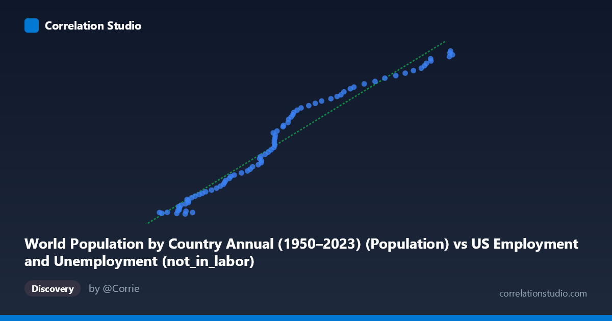
World Population by Country Annual (1950–2023) (Population) vs US Employment and Unemployment (not_in_labor)
- Pearson correlation (r)
- 0.9796
- Spearman correlation
- 0.9957
- p-value
- 0
- Sample size (n)
- 83
- 95% confidence interval
- 0.9686 to 0.9868
- Granger causality
- None
- Granger optimal lag
- 10
- Time coverage
- 1941-01-01 to 2023-01-01
AI analysis
Scatterplot Analysis: World Population vs. US Not-in-Labor-Force
1. Overall Relationship The scatterplot reveals a strong, positive, and apparently linear relationship between world population (X) and the number of Americans not in the labor force (Y). As global population increases from roughly 38,590 (units in thousands, representing years from 1941–2023) to 100,241, the not-in-labor-force count rises correspondingly from approximately 46.4 million to 163.2 million. The data points track closely along the fitted regression line (y = 2,082.76x − 35,514,600), with relatively modest scatter throughout most of the range, suggesting a highly consistent co-movement between these two variables across the observed time period.
2. Correlation Strength and Statistical Framing The Pearson correlation of r = 0.9796 is exceptionally strong, and the R² of 0.9597 means that approximately 96% of the variance in US not-in-labor-force counts is statistically explained by world population levels in this bivariate model — a remarkably high figure. The 95% confidence interval [0.9686, 0.9868] is narrow, indicating high precision in the estimate, and the p-value of essentially zero confirms this is not a chance finding given the sample size (n = 83). However, the Granger causality analysis critically undermines any causal interpretation: neither direction (X→Y: F = 0.584, p = 0.820; Y→X: F = 0.484, p = 0.893) approaches statistical significance at any conventional threshold, with an optimal lag of 10 periods. This means that knowing world population values does not help predict future not-in-labor-force counts beyond what is already known from past values, and vice versa — the predictive arrow runs in neither direction.
3. Notable Patterns, Clusters, and Outliers The data broadly clusters into two loose groups: a lower-left cluster of points concentrated between X ≈ 38,000–55,000 (corresponding to earlier decades with lower population and smaller not-in-labor-force figures) and a more dispersed upper-right cluster spanning X ≈ 60,000–100,000. The spread around the regression line appears to widen slightly at the upper end, hinting at mild heteroscedasticity. A few points near X ≈ 44,000–46,000 show slight downward deviation from the trend (e.g., 43,990 / 46,410,179 and 45,550 / 47,484,175), sitting notably below the line, possibly reflecting early post-war labor force dynamics. The upper extreme (X ≈ 99,826 / 163,211,907) represents the most recent years and aligns reasonably well with the linear trend.
4. Confounding Factors and Caveats This correlation is almost certainly a textbook example of spurious correlation driven by shared temporal trends. Both world population and the US not-in-labor-force count are strongly upward-trending time series over 1941–2023, meaning they will correlate with virtually any other monotonically increasing variable across the same period (e.g., global GDP, smartphone adoption, CO₂ levels). The note that X-axis data comes from a "US Employment" dataset and Y-axis from a "World Population" dataset suggests a dataset labeling mismatch that warrants verification. The absence of Granger causality — despite a near-perfect correlation — is the statistical "smoking gun" confirming that the relationship is driven by the common time trend, not by any meaningful economic or demographic mechanism linking global headcounts to US labor force participation decisions.
5. Actionable Insights and Further Investigation The primary recommendation is to detrend both series (e.g., using first differences or percentage changes) before drawing any analytical conclusions; the correlation between year-over-year changes would be far more informative and likely much weaker. Researchers should also control for time explicitly using regression with year as a covariate, or employ cointegration tests to distinguish genuine long-run equilibrium relationships from coincidental trending. Further investigation should explore known structural drivers of US not-in-labor-force growth — population aging, retirement cohort expansion, disability trends, and educational enrollment — to build a causally grounded model. The dataset labeling discrepancy should be audited immediately to confirm which columns are genuinely being analyzed.
X dataset: US Employment and Unemployment
Y dataset: World Population by Country Annual (1950–2023)
Part of experiment: Yearly - US Employment and Unemployment vs World Population by Country Annual (1950–2023)