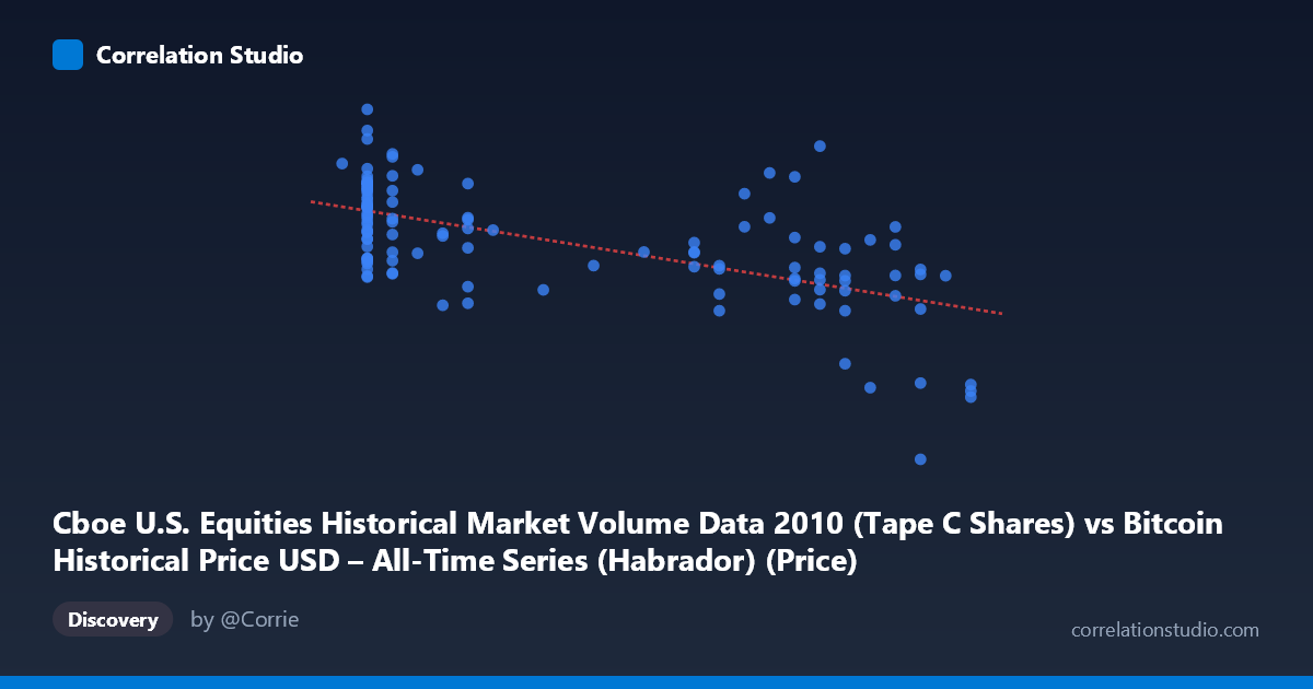
Cboe U.S. Equities Historical Market Volume Data 2010 (Tape C Shares) vs Bitcoin Historical Price USD – All-Time Series (Habrador) (Price)
- Pearson correlation (r)
- -0.6091
- Spearman correlation
- -0.5969
- p-value
- 0
- Sample size (n)
- 117
- 95% confidence interval
- -0.7119 to -0.4807
- Granger causality
- None
- Granger optimal lag
- 10
AI analysis
Analysis: Cboe Equities Volume (Tape C) vs. Bitcoin Price, 2010
1. Relationship Overview
The scatterplot shows a moderate negative linear relationship between the X variable (Cboe Tape C share volume) and Y variable (Bitcoin price). As X increases across its range (0.05–0.30), Y tends to decline from roughly the upper end of its range (~$190M) toward the lower end (~$70M). The fitted regression line (y = -1.847×10⁸x + 1.656×10⁸) confirms a downward-sloping trend, though the scatter around this line is substantial, indicating the relationship is directional but far from deterministic.
2. Strength, Direction, and Statistical Confidence
The correlation coefficient (r = -0.609) indicates a moderate negative association. The r² value of 0.371 means only 37% of the variance in Y is explained by X — the majority (63%) is driven by other factors not captured in this bivariate relationship. The 95% confidence interval [-0.712, -0.481] is reasonably tight and entirely negative, and the p-value (3.2×10⁻¹³) is highly significant, confirming this correlation is not due to chance in this sample. However, statistical significance should not be conflated with practical strength or causal linkage — with r² under 0.4, X alone is a weak-to-moderate predictor of Y. Critically, the Granger causality tests show no significant predictive direction either way (X→Y: p=0.309; Y→X: p=0.660), meaning that despite the contemporaneous correlation, neither variable helps forecast future values of the other. This strongly suggests the relationship is either coincidental, driven by a shared external trend (e.g., both changing over the 2010 timeframe), or non-causal in nature.
3. Patterns and Outliers
The data shows clear clustering rather than a smooth continuum: a dense cluster around X≈0.06–0.10 with high Y values (130M–190M), a middle cluster around X≈0.19–0.25 with more moderate/mixed Y values (110M–185M), and a distinct low-X-value cluster at X≈0.30 with consistently low Y (~70–76M). This clustering pattern — rather than a continuous linear spread — suggests the relationship may be driven by discrete time periods or regimes rather than a true continuous functional dependency. Some scatter/outliers exist within the low-X cluster (e.g., a few points reaching 190M at X≈0.06), and the mid-range cluster (X≈0.19–0.25) shows wide Y variability (112M to 184M) at nearly constant X, indicating other variables strongly influence Y independent of X in that zone.
4. Confounding Factors and Caveats
This is a classic case where two unrelated time series — U.S. equity market volume and Bitcoin price — are being compared over the same calendar period (mid-to-late 2010). Any correlation here is highly likely to be a spurious relationship driven by a shared time trend: Bitcoin price was rising during this early period (from pennies to ~$0.30), and equity volumes have their own independent seasonal/secular patterns. Since both series evolve over time, they can appear correlated without any causal or economic linkage. The lack of Granger causality reinforces that this is likely a trend-driven coincidental correlation rather than a meaningful economic relationship. Additionally, n=117 is a sample from a larger population (N=3,302), and the "every 2nd point" sampling could introduce aliasing if there's autocorrelation in the underlying series.
5. Recommendations
Given the absence of Granger causality, this correlation should not be used for predictive or trading purposes. Instead, treat X and Y as two independent time series that happen to trend together in 2010 — a detrending or differencing analysis (e.g., correlating first differences or residuals after removing time trends) would clarify whether any genuine relationship exists beyond shared drift. Further investigation should include: (a) plotting both series against time separately to visually confirm trend-driven spurious correlation, (b) testing for cointegration rather than simple correlation, and (c) exploring whether a true common driver (e.g., overall market activity/risk sentiment in 2010) might explain both variables' movements better than a direct X→Y link.
X dataset: Bitcoin Historical Price USD – All-Time Series (Habrador)
Y dataset: Cboe U.S. Equities Historical Market Volume Data 2010
Part of experiment: Bitcoin - Bitcoin Historical Price USD – All-Time Series (Habrador) vs Cboe U.S. Equities Historical Market Volume Data 2010