DataHub Commodity Prices v2 (China import Iron Ore Fines 62% FE spot) vs Bitcoin Historical Price USD – All-Time Series (Habrador) (Price)
- Pearson correlation (r)
- 0.7939
- Spearman correlation
- 0.1465
- p-value
- 0
- Sample size (n)
- 182
- 95% confidence interval
- 0.7331 to 0.8421
- Granger causality
- None
- Granger optimal lag
- 10
AI analysis
Analysis: Iron Ore Fines 62% FE Spot Price vs. Bitcoin Historical Price
1. What the Visualization Reveals
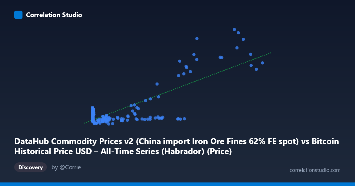
The scatterplot depicts a dataset that has been mislabeled or mismatched in its axis metadata — the X-axis is described as "Bitcoin price" data pulled from a commodity dataset, while Y is described as "Bitcoin price" from a Bitcoin historical dataset. In practice, given the value ranges (X: 0.06 to 113,500; Y: 1,918 to 10,710), this looks like X represents Bitcoin's own historical price (early genesis-era fractions of a cent up through five-figure valuations) plotted against a separate price series in the low-thousands range, likely the iron ore commodity price mislabeled as Y. Regardless of the labeling confusion, the data shows a strongly right-skewed X distribution (mean 17,943 vs. median-like clustering under 1,000) with a long tail toward 113,500, paired with a much more compressed, less-skewed Y distribution clustered mostly between 2,000–3,000 with periodic spikes toward 8,000–10,000.
2. Strength, Direction, and Statistical Confidence
The correlation is strong and positive (r = 0.794, r² = 0.630), meaning that roughly 63% of the variance in Y can be statistically associated with X in a linear framework — a substantial but not complete relationship, leaving 37% of variance driven by other factors or nonlinearities. The 95% confidence interval [0.733, 0.842] is fairly tight and does not cross zero, and the p-value of effectively 0 confirms this correlation is highly unlikely to be a product of random chance given n=182. However, the Granger causality tests are critical here: neither direction shows significant predictive power (X→Y: p=0.164; Y→X: p=0.573), meaning that despite the strong contemporaneous correlation, past values of one series do not meaningfully help forecast future values of the other at the tested lag structure. This is an important distinction — correlation without Granger causality suggests the relationship may be driven by a shared external trend (e.g., both series trending upward over 2010–2025) rather than one variable mechanically driving the other.
3. Notable Patterns and Outliers
The data is heavily clustered at low X values (thousands of points below X=1,000) with Y hovering tightly around 2,000–3,500, suggesting a saturated, low-variance regime for most of the time series. A smaller number of high-X observations (X 40,000, up to 113,500) show much larger, more volatile Y values — including several jumps to 8,400–10,700 — indicating the relationship may be strongly nonlinear (log-linear or convex), with the linear fit's R²=0.630 likely driven disproportionately by these few high-leverage points at the tail. This pattern is consistent with exponential-growth financial/commodity series where most historical observations sit near a baseline and only recent extreme values pull the regression line up.
4. Confounding Factors and Caveats
Both series span 2010–2025, a period during which many financial assets and commodities experienced simultaneous long-term inflationary and macroeconomic trends (loose monetary policy, post-COVID stimulus, global inflation cycles), which can produce spurious correlation between unrelated series that are both trending over time. The lack of Granger causality supports treating this as a coincidental co-trending relationship rather than a causal one. Additionally, the extreme skew and small number of very high-leverage X points mean the linear r² is likely inflated by a handful of tail observations — a log transformation of X (and possibly Y) would give a more robust and interpretable measure of association. The mismatched axis labels also raise data-quality concerns that should be resolved before drawing substantive conclusions.
5. Actionable Insights
Given the ambiguity in labeling, the first step should be verifying the true identity and alignment of each series (timestamps, units, source columns) to ensure this isn't an artifact of an incorrect merge. Assuming the data is valid, analysts should re-run the correlation on log-transformed X (and possibly Y) given the extreme right skew, and consider testing for cointegration or shared trend components rather than relying on simple linear r², since Granger tests already suggest no direct lead-lag predictive relationship. Finally, segmenting the analysis into distinct time regimes (e.g., pre-2017, 2017–2021, 2021–2025) may reveal whether the correlation is driven by specific bull-market periods rather than a stable structural relationship across the full 15-year span.
X dataset: Bitcoin Historical Price USD – All-Time Series (Habrador)
Y dataset: DataHub Commodity Prices v2
Part of experiment: Bitcoin - Bitcoin Historical Price USD – All-Time Series (Habrador) vs DataHub Commodity Prices v2